Cross-subsidization of Bad Credit in a Lending Crisis

NBER WORKING PAPER SERIES

CROSS-SUBSIDIZATION OF BAD CREDIT IN A LENDING CRISIS

Nikolaos Artavanis

Brian Jonghwan Lee

Stavros Panageas

Margarita Tsoutsoura

Working Paper 29850

http://www.nber.org/papers/w29850

NATIONAL BUREAU OF ECONOMIC RESEARCH

1050 Massachusetts Avenue

Cambridge, MA 02138

March 2022

We have benefited from comments by Claudia Robles-Garcia, Sascha Steffen (discussant), and

participants at AFA, AEA, Frankfurt School, Columbia Business School, RCEA, and ECB.

Tsoutsoura gratefully acknowledges financial support from the Fama-Miller Center for Research

in Finance at Chicago Booth. The views expressed herein are those of the authors and do not

necessarily reflect the views of the National Bureau of Economic Research.

NBER working papers are circulated for discussion and comment purposes. They have not been

peer-reviewed or been subject to the review by the NBER Board of Directors that accompanies

official NBER publications.

quoted without explicit permission provided that full credit, including © notice, is given to the

source.

Cross-subsidization of Bad Credit in a Lending Crisis

Nikolaos Artavanis, Brian Jonghwan Lee, Stavros Panageas, and Margarita Tsoutsoura

NBER Working Paper No. 29850

March 2022

JEL No. E43,E44,G01,G21,G3

ABSTRACT

We study the corporate-loan pricing decisions of a major Greek bank during the Greek financial

crisis. A unique aspect of our dataset is that we observe both the interest rate and the “breakeven

rate” of each loan, as computed by the bank’s own loan-pricing department (in effect, the loan’s

marginal cost). We document that low-breakeven-rate (safer) borrowers are charged significant

markups, whereas high-breakeven-rate (riskier) borrowers are charged small and sometimes even

negative markups. We rationalize this de-facto cross-subsidization of riskier borrowers by safer

borrowers through the lens of a dynamic model featuring depressed collateral values, impaired

capital-market access, and limit pricing.

Nikolaos Artavanis

Virginia Tech

1016 Pamplin Hall

Blacksburg, VA 24061

[email protected]

Brian Jonghwan Lee

Columbia Business School

665 West 130th Street

New York, NY 10027

[email protected]

Stavros Panageas

Anderson School of Management

University of California, Los Angeles

110 Westwood Plaza

Los Angeles, CA 90095-1481

and NBER

[email protected]

Margarita Tsoutsoura

SC Johnson College of Business

Cornell University

Ithaca, NY 14853

and NBER

[email protected]

1 Introduction

A common concern among macroeconomi sts and ﬁnancial economists is that the cr ed i t

market is distorted duri n g a ﬁnancial crisis. The concern can be summarized as follows:

banks may be reluctant to terminate loans, because of depressed collateral values. As a

result, worse-performing ﬁrms are charged interest rates below a “fair rate” in order to

keep these ﬁrms “aﬂoat.” In an eﬀort t o make up the losses, banks overcharge healthy and

growing ﬁrms that d on ’ t have many funding alternatives during a crisis. The result is a

de-facto cross-subsidization of weaker ﬁrms by stronger ﬁrms, wh i ch misallocates credit a n d

prolongs the ﬁna nci a l crisis.

A common challenge in testing this cross-subsid i za ti o n hypothesis is determining whether

a given loa n i s upcharged or is extended at preferential terms. Such a determination requi r es

knowledg e of the “fair” or “breakeven” rate for that loan. By breakeven rate we mean the

interest rate that would make the lender break even, tak i n g into account the lender’s fun d i n g

rate and operating costs, as well as the borrower’s probability of default times the expected

loss upon defau l t (taking into account coll a t era l ) and any regulatory charges associated with

the loan. In eﬀect, the breakeven rate is the marginal cost of the loan from the lender’s

perspective. To address this limitation, the l i ter a t ure typically imputes the breakeven rate

in some indirect manner.

As a resu l t , the theory ends up being test ed jointly with the

ndirect imputation method, resulting in a “joint hypot h esi s” problem.

In this paper, we provide direct evidence in support of th e cross-subsidizati on hypothesis,

by using a dataset that contains loan-level breakeven rat es. The dataset pertains to the large

corporate portfo l i o of a major Greek bank at the height of the recent Greek ﬁnancial crisis.

The unique a spect of the dataset is th at besides loan-level info rm a t i on (actual interest rate,

maturity) and ﬁrm-level informatio n , we also observe the loan-level breakeven rate that

the bank’s own loan-pricing department supplies to the loan managers ahead of the loan

negotiations. This allows a direct observation of the diﬀerence between the actual and

breakeven rate, which we r efer to as the “markup” of each loan.

Our main ﬁnding is th a t the bank charges an interest rate well above the breakeven

We summari ze some indirect approaches in our discussion of the literature.

rate to comparatively safe borrowers (low-breakeven-ra te borrowers). By contrast, the bank

charges a zero, and sometimes even negat i ve, marku p to its riskier loans (high-breakeven-

rate borrowers). Importa ntly, because the loans in our sample are performin g loans, we are

able to show that thepatt er n of cross-sub si d i za ti o n app l i es even within the set of performing

loans, and our conclusions are not conﬁned to a narrow comp ar i so n between performing and

non-performing loan s.

We nex t describe in greater detail the theoretical motivation behind our tests, the context

of our empirical analysis, and our key ﬁndings.

To provide a framework for our empirical results, we start by building a dynamic corpo-

rate ﬁ n an ce model. The model is tailored to capture the speciﬁc institution al and historical

context o f o u r empirical analysis, but its key features are fairly standard and broadly used in

the literature. In the m odel, a borrower needs funds and a competitive b a n k provides them.

We study this model during a “crisis” and a “post-crisis” regime. In the p ost -cr i si s regime,

the bank has friction-less access to capital markets and the collateral values of capital are

high eno u gh that terminat i n g low proﬁtability borrowers is p r o ﬁ t ab l e. By contrast, when

the economy is in a crisis, we assume (a) the bank loses its frictionless access to capital

markets and has limited or no access to new capital and (b) the collateral values of capital

are temporarily depressed.

We sh ow loan pricing diﬀers for low-proﬁtability and high-proﬁtab i l i ty borrowers. The

interest rate for low-proﬁtability borrowers is disconnected — and may even be lower than

— the loan’s marginal cost, because of the real option to wait unti l either collateral values

rebound or the ﬁrm productivity rebounds. For such borrowers, the bank simply extracts

what each low-proﬁtability borrower can aﬀord to pay. At the same time, the reluctance

of competitor banks to terminate their own low-productivity projects and their ina b i l i ty to

raise new capital in i nternational ﬁnancial markets implies that high-pro ﬁ ta b i l i ty borrowers

cannot be poached easily by competitors. Thus, they can be charged a markup, up to

the point where competitor banks are ind i ﬀer ent between poach i n g the loan or not (“limit

pricing”).

The theoretical model makes two basic predictions: First, a cross-sectional regression of

actual loan rates on their breakeven rates should have a coeﬃcient less than one, reﬂecting

that ﬁnancial l y healthier borrowers are upcharged, relative to weaker ones. (We label this

prediction an imperfect “pass through” of the br eakeven rate to the actual rate.

) Second,

pass through should be asymmetric: The pass-throu g h coeﬃcient should be higher for high-

proﬁtability ﬁrms, whose loans are priced according t o a limit prici n g rule, and weaker for

ﬁrms whose loans are priced according to what th e borr ower can aﬀord to pay.

We test these predictions using a dataset that includes the universe of l a rg e-ﬁ r m loans

of a major, systemic bank in Greece. We expl o i t a regulatory reform in the Greek b an k i n g

system that required ﬁnancial instituti on s to develop new, transparent loan -l evel pricing

guidelines. The requirement was imposed by the the monitoring instituti o n s of the Greek

MoU (Memorandum of Under st a n d i n g) following the recapitalization of Greek banks in 2012.

In response to these mandates, each systemic bank had to develop its own pri ci n g model

independently, adhering to two requirements. Fi r st , the pricing model had to be formulaic

and data d r i ven (i.e., reﬂect balance-sheet information rat h er than subjective assessments),

follow the Basel gu i d el i n es and be used to com p u t e capital charges at the loan level. Second,

it had to be applied uniformly to all loans of th e same class with common parameters for no n -

ﬁrm-speciﬁc variables. The ultimate output should be a loan-level breakeven rate, deﬁned

as the interest rate that makes the bank break even on the loan. The new pricing model

went into eﬀect in 2015, approximatel y two quarters before the peak of the Greek ﬁnancial

crisis. Importantly, after the introduction of the new pricin g guidelines, loans extended with

interest rates below the breakeven rate required internal approval that stated the justiﬁcation

for the discount.

The introduction of the new pricing guidelines has a profound impact on loan pricing.

Loan managers heed the new guidelines a n d start “p assi n g through” the breakeven ra tes

to the loans that are initia ted or renewed. Indeed , the breakeven rate appears to be the

only variable that matters for loan pricing after the introduction of the new prici n g guide-

lines. This ﬁnding is in contrast to the pre-guidel i n e period, where the (ex-post calculated)

breakeven rate plays n o role for loan pricing. At the same t i m e, variables capturing non-

economic factors (polit i ca l connections of board members, du m my variables that in d i cat e a

A mathematically equivalent formulation of the imperfect pass-through hypothesis is that the diﬀerence

between the actual and breakeven rate (the markup) is decreasing in the breakeven rat e.

tightl y held ﬁrm, etc.) seem to matter for loan pricing during the pre-gui d el i n e period, but

are driven out post-guid el i n e.

Having established that the new pricing guidelines weren’t simply ignored, but instead

had a profound impact on loan pricing, we test for imperfect pa ss-t h ro u g h of th e brea keven

on the actual rate aft er the introduction of the new pricing guidelin es. Consistent wit h our

model, the coeﬃcient o f a regr essi o n of th e actual rate on the breakeven rate is al ways below

one, implying markups are decreasing in the breakeven rate. This ﬁ n d i n g is pervasive. We

even obser ve several instances in which loans are extended at below-breakeven rates, with

loan managers choosi n g to go through the arduous internal-app r oval process.

We also document a pricing asymmetry. The pass-through coeﬃcient (controlling for

time an d ﬁrm ﬁxed eﬀects) is about 0.4 for rel a ti vely safe borrowers (borrowers with below-

median break-even rates on the da t e of the introduction of the new pricing guidelines). The

same coeﬃcient i s essentially 0 for rel at i vely risky borrowers (borrowers with above-median

break-even rates on the date of the introducti o n of the new pricing scheme). This ﬁnding

is consistent with the view that the pricing decisions for the riskier borrowers are decoup l ed

from th e riskiness of their loan. Instea d , they are mostly dictated by the borrower’s ability

to pay, consistent with our theoretical mod el .

Next, we examine possible alternative interpretations of our results. We investigate

whether the source of the imperfect pass-through is due to managers’ possessing some su-

perior informat i on on the long-term prospects of the ﬁrm, which induces them to moderat e

the impact of th e breakeven rate on their loan-p r i ci n g decisions. Utilizing a test analogous

to Chiappor i & Salanie (2000), we test whether a low (h i g h ) markup correlates with subse-

uent improvement (deterioration) in the borrower’s credit rating. We ﬁnd that the markup

has no abi l i ty to predict future changes in the borrower’s credit rating — after controlling

for the cur r ent credit rating. Therefore, the source of the imperfect pass-through is not

due to managers’ possessing some superior inform a t i on on the lon g -t erm prospects of the

ﬁrm, which induces them to moderate the impact of the breakeven rate on th ei r loan-pricing

decisions. Our results are also not driven by lo a n managers choosing to pass through only

the component of the breakeven rate that is narr owly linked with the regulatory charge of

the loan. Isolating the component of the breakeven rate that corresponds to the regulatory

charge of each loan, and including it as a separate regressor (alongside the breakeven rate)

does not change our results.

Our results relate to several strands of the l i t era t u r e. The literature on zombie lend-

ing (Peek & Rosengren (2005); Caballero, Hoshi & Kashyap (2008); Giannetti & S i m o n ov

(2013)) has exami n ed the widespread practice by Japanese banks in th e 9

0s to provide credit

to insolvent ﬁrm s. Much of the liter at u r e sh i ft ed its focus to Europe dur i n g t h e sovereign

debt crisis (Ach ar ya, Imbierowicz, Steﬀen & Teichma n n (2020); Acharya, Eisert, Euﬁnger &

rsch (2019); Acha r ya, Crosignani, Eisert & Euﬁnger (2020); Schivardi, Sette & Tabellini

(2021); Blatt n er , Farinha & Rebel o (2019); Banerjee & Hofmann (2018); McGowan, Andrews

Millot (2018); Albertazzi & Marchetti (2010)). In a contempora n eou s paper, Faria-e Cas-

ro, Paul & Sanch´ez (2021) provide evidence of “evergreening” in the US using supervisor y

data from the Federal Reserve. As mentioned earlier, our dataset allows for a direct test of

the cross-subsidi zat i o n hypothesis, without having to rel y on some indirect inference for the

“fair” (or “breakeven”) rate of each lo a n .

In addition, although related to the liter a tur e

n zombie lending, our paper is not just about zombie loans. Because we can observe the

markup of each loan, we are able to document a broader pattern of cross-subsidization of

riskier borrowers by safer borrowers across performing loans.

A large literature investigates “cross-subsidization”, especially in asymmetric-information

settings. Puelz & Snow (1994) and Chiappori & Salanie (2000) prov i d e early examples o f

esting for cross-subsidization from safe consumers to risky consumers in the auto insuran ce

market. Similar notions of cross-subsidizati o n have been examined in other areas including

the mortgage ma r ket (Hurst, Keys, Seru & Vavra (2016); Gambacorta, Guiso, Mistrulli,

ozzi & Tsoy (2019)); student loans ( Ba chas (2019)), and health insurance (Finkelstein

(2004), Finkelstein & McGarry (2006), Aizawa & Kim (2018)). In a recent paper, Nelson

(2020) shows a regulatory ch an g e in the US credit card ma rket restric

ted cross-sectional

passthrough across credit card consumers, thu s providing cheap er credit to risky consumers

while safe consumers received overpr i ced credit. Our notion of “cross-subsidization” diﬀers

from the above literature in that it pertains to knowingly charging diﬀerent markups to clients

Prior research on zombie ﬁrms examined interest cover age ratio, credit rating, delinquency, unreported

loss, and accounting variables to ascertain whether a bank subsidized a given ﬁrm.

who are observably di ssi m i l ar (as reﬂected in their diﬀerent breakeven rates), as opposed to

the cro ss-su b si d i zat i on that arises when borrowers who a re observably similar (but dissimilar

on unobservables) are pooled together and charged the same pri ce.

Screening models of cross-subsidization provide an alternative framework to ours to cap-

ture cross-sub si d i zat i o n of observably dissimilar clients, as reveal ed by the client’s choices.

Several reasons seem to suggest su ch a framework may not be well suited for the speciﬁc

context we study in this paper. First, such model s do not contain clear implications about

the pattern of cross-subsidizati o n . Oligopolistic screening introdu ces a ma r ku p , but leads to

ambigu o u s prediction s as to whether the markup per dollar loaned should be increasing or

decreasing with borrower riskiness.

Second, i n such models, the markup is typically posi-

ive across a l l credit qualities,

whereas in our data , we observe several instances in which

loan managers extend loans at below-breakeven rates, hinting at the presen ce of a “real op-

tion.” Third, as mentioned earlier, in section 7.1, we perform a test similar in spirit to the

symmetric-information test of Chiap pori & Salanie (2000)

and ﬁnd that the actual interest

rate on a loan does not appear to have superior ex -post predictive abi l i ty about a bo rr ower’s

future prospects.

Due to its dy n a m i c nature, our model resembles the large banking literature on relation-

ship lending.

Given the focus on the Greek ﬁnancial crisis, t h e p a per also co

ntribu t es t o the

literature on i m p ai r ed ﬁnancial intermediation in the context of the European Sovereign Debt

Crisis (Acharya, Drech sl er & Sch n ab l (2014); Ach a r ya, Eisert, Euﬁnger & Hirsch (2018);

Acharya, Imbierowicz, Steﬀen & Teichmann (2020)). Several articles examine the relation-

hip between bank market power and interest rate pass through (Hannan & Berger (1991);

Berger & Udell (1992); Neumark & Sharpe (1992); Zenteﬁs (2019)). For instance, Sch ar fst ei n

For instance, the oligopolistic screening model of the lending market by Villas-Boas & Sch mi dt -M oh r

(1999) has parameter-dependent implications about whether the markup should be higher or lower for riskier

loans. In an industrial organization framework similar to the seminal Mussa & Rosen (1978) non-linear

pricing framework, Rochet & Stole (2002) show that as competition intensiﬁes, their oli gopolistic model

converges to a ﬁxed fee model, independent of revealed borrower characteristics.

See, for example,Villas-Boas & Schmidt-Mohr (1999).

Chiappori & Salanie (2000) test for a correlation between ex-ante choices of auto-insurance cover

age and

ex-post accidents. In our context, we test whether a seemingly low interest rate tends to predict positive

revisions to a bor r ower’s future rating.

See, for example, Diamond (1991); Rajan (1992); Petersen & Rajan (1994); Boot & Thakor (2000);

Hachem (2011).

& Sunderam (2016) show how bank market power can limit mon et a ry -policy tr a n smission

to mor t g ag e rates. The noti o n of limited pass-through in th ese papers is diﬀerent fro m that

in our paper. For us, limited pass-through is primaril y a cross-sectional no t i on : it refers to

a less than one-for-one relation between the actual and brea keven rate across diﬀerent loans

at the same point in time.

2 Model

In this sect i on , we propose a stylized model to aid the interpr

etation of our empirical

results. The model contains several elements th at are meant to capture th e speciﬁc economic

context of Greek banks and borrowers during the time period of our study. Al th o u g h a few

of the modelli n g choices are m o t i vated by the speciﬁc historical experien ce of Greece, t h e

assumptions of the model are standard and would apply to any banking system in crisis.

In particular, we con si d er a basic dynamic corporate ﬁnance problem whereby a lender

and a borrower split the cash ﬂows of a project during times of “cri si s” and “post crisis.”

Our focus is on the state of crisis. We make three assumptions about the crisis, motivated by

the ci rcu m st a n ces Greek ﬁrms and banks faced during ou r sample period: (a) Greek banks

had limited access to international capit al markets, (b) collateral values of all projects were

depressed during this time period, and ( c) shar eh ol d er s had essentially no abili ty to perfor m

equity injections.

To ﬁx ideas, we star t by presenting ﬁrst the post-crisis version of the model and then

work backwards to present the model solution during the time of the cri si s. Speciﬁcal l y, we

assume that the economy is in a state of crisis at time 0. At some random, exponentially

distributed time τ, the eco n omy transits to th e post-crisis state. The arrival of this event

occurs with a hazard rate ρ per unit of time dt. Throughou t , sup er scr i p t “c” denotes a

variable during the state of crisis.

2.1 Post crisis

Throughout, we assume that a ty p i ca l ﬁrm produces a stochastic cash-ﬂow process π

per unit of capital and per unit of ti m e d

t. For simplicity, we assume (a) each ﬁrm only

uses one unit of capital, and (b) this cash-ﬂow process takes two values according to an

(idiosyncratic and ﬁrm-speciﬁc) Markov regime-switching process.

The cash -ﬂ ow process

of ﬁrm i takes th e value π

when the ﬁrm is in regime H a

nd the value π

when the ﬁrm

is in regime L. The hazard rate of l eaving regi m e H and transitioning to regime L is equal

to p

, and the hazard rate of the reverse transition is p

. The transitions between the two

regimes are independent across ﬁrms. Moreover, ﬁrms can diﬀer in terms of the parameter s

, p

, π

,and π

ile keeping in mind that t h e parameters p

, p

, π

, and π

can diﬀer across ﬁrms,

ereafter, we drop the subscript i and u se the simpler notation p

, p

, π

, and π

In the post-crisis economy, banks are perfectly competitive and can borrow and lend

freely at the rate r

∗

in international capital markets. The (representative) ban

k provides the

unit of the capital stock to the ﬁrm an d in exchange obtains a cash-ﬂow stream R

, which

depends on ﬁrm i and the proﬁtability regime j ∈ {H, L} of ﬁrm i. We normalize the price

of one unit of the capital st ock to 1. At any point in tim e, th e bank can liqu i d a t e the capital

stock and obtain a value C

∗

< 1. I

n oth er words, the diﬀerence between the price of capi t a l

and its liquidated value, 1 − C

∗

> 0, is the deadweight cost of bankruptcy. To economize

notation, we drop the subscript i and write R

and C i

nstead of R

and C

(respectively).

Throughout, we abstract from corporate cash accumulation by assuming shareholders

have a suﬃciently high discount rate λ.

For simplicity, we also suppress equity issuance by

ssuming shar eh ol d er s cannot inject any additional equity to the ﬁrm, and hence, R

≤ π

for j ∈ {H, L}. Finall y, all debt is short term (i.e., needs to be constantly rol l ed over) and

the bank can withdraw th e un i t of capital at any time. Similarly, companies can reﬁnance

their loans at no cost by repaying the current bank in the full amount and obtaining a new

loan from another competi t i ve bank.

The value of a deb t contract V

from the perspective of a bank obey s a standard asset-

ricing rel at i o n sh i p . When t h e proﬁtability of the ﬁrm is in regime H, the value of the debt

Allowing mu l t i pl e p r oﬁt ab i li ty r egimes or allowing ﬁrms to choose th e scal e of t hei r capital is strai ght-

forward, but is immaterial for the purposes this paper. Abel & Panageas (2020a) present a version of this

model that allows the ﬁrm to vary its scale by adjusting the units of the capital stock.

Abel & Panageas (2020b) study a version of this model th at allows for cash accumulation and show a

igh-enough shareholder discount rate leads to no cash accumulation.

contract is

|{z}

Interest paid to the bank

+ p

max{V

, C

∗

} − V



{z }

expected capital loss upon regime change

= r

∗

|{z}

required rate of return

(1)

imilarly, the pricing equation when the ﬁrm i s in regime L is

|{z}

Interest paid to the bank

+ p

− V



{z }

expected capital gain upon regime change

= r

∗

|{z}

required rate of return

. (2)

Because banks are competitive, it must be the case that both V

≤ 1

and V

≤ 1.

Otherwise, a competi t or bank can oﬀer to reﬁn an ce the loan, whose face value is 1. At the

same t i m e, a bank will not initiate a loan unless it makes non-negative proﬁts, which leads

to V

= 1, a

nd hence, by equation (1), we have

= r

∗

+ p

1 − max{V

, C

∗

}



. (3)

We assume

> r

∗

+ p

(1 − C

∗

) , (

which implies R

< π

, an d hence, the bank can feasib l y charge t h e interest rate R

that

allows it to break even.

Using V

= 1 inside ( 2 ) gives

+ p

1 − V



= r

∗

(5)

he bank will ﬁn d it optimal t o liquidate the ﬁrm whenever V

< C

∗

. T

he maximum

possible value of V

is obtained by setting R

= π

, in which case equation (5) becomes

+ p

∗

+ p

. (6)

Further, we assume

∗

+ p



∗

− p

, (

and therefore, (6) implies V

< C

∗

, which in turn implies liquidating the ﬁrm in regime

L is optimal. We summarize the above discussion in the following proposition

Proposition 1. Assume conditions (4) and (7) hold. Then,

= r

∗

+ p

(1 − C

∗

) , (

and the ﬁrm gets liquidated once it enters the low-proﬁtability regime L.

The post-crisis interest rate (8) is intuitive and familiar. The bank charges its own

unding rate r

∗

along with an additional compon ent reﬂecting the probability of default p

times the loss upon default (1 − C

∗

). No

te that because we have allowed p

to diﬀer across

ﬁrms, so will the interest rate R

that the bank charges t o diﬀerent ﬁrms, dependin g on

each ﬁrm’s default risk.

2.2 Crisis

The focus of our analysi s is on the state of crisis. The crisis-version of the model is

identi cal to the post-crisis versio n , except that: (a) collateral values are lower during the

crisis period, so that liquid at i o n of a ﬁrm al l ows the bank to recover onl y C < C

∗

per unit of

apital, and (b ) banks have limited access to international capital markets; therefore, they

have to ﬁn an ce new projects using their internal funds. This second assumption is mostly for

expositional ease and can be relaxed to al l ow banks to have costly access to capital markets,

as we discuss at the end of this section. Although not essential for our results, we also allow

the required rate of return of bank sh a reh o l d er s (r) to diﬀer from its post-crisis level (r

∗

) .

etting V

H,c

L,c

) denote th e value of debt when a gi ven ﬁrm i i

s in the H (resp. L)

regime and the economy is in the crisis state “c,” we obtain the pricing equation:

H,c

+ p

L,c

− V

H,c



+ ρ

1 − V

H,c



= r

H,c

. (9)

The ﬁrst two terms on the l eft -h a n d side of (9) are the same as dur i n g the pre-crisis

eriod, namely, the sum of the interest charged by the ba n k, R

H,c

, p

lus the expected capital

loss upon transition to the low-proﬁtability regime, p

L,c

− V

H,c



. The third term, reﬂects

the expected change in the value of the debt upon transition to the post-crisis state, which

is the prod u ct of the transition hazard ρ times the change i n the value of debt, 1 − V

H,c

Similarly, for a ﬁrm that ﬁnds itself in regime L, the debt-pricing equation is

L,c

+ p

H,c

− V

L,c



+ ρ

∗

− V

L,c



= r

L,c

. (10)

Clearly, a bank will not ﬁnd it proﬁtable to liquidate a loan as long as V

L,c

≥ C

The assumption that banks have to ﬁnance projects from i nternal funds limits compe-

tition between banks for ﬁr m s in the H regime. To poach a borrower in the H r eg i m e, a

rival bank has t o liquid a t e

of its existing loans, so that it can raise the face value of the

oan it is poaching,

C = 1. Clearly, the rival bank ﬁnds it proﬁtable to engage in such

poaching only if V

H,c

≥

, where D is the minimal value V

L,c

across all debt contracts that

the rival bank is ﬁnancing. (The heterogeneity of the parameters p

, p

, π

, e

tc. across

ﬁrms implies V

H,c

and V

L,c

diﬀer a cr os s ﬁrms). Because V

L,c

≥ C for any debt contract of

any bank, it must be the case that

≥ 1.

In summary, unlike in the post-cri si s regime, where the no-poaching condition amou nts

to V

= 1, d

uring a crisis, the no -poaching condition leads to V

H,c

, where

≥ 1. We

obtain the following proposition.

Proposition 2. Assume conditions (4) and (7) hold, and in addition, assume

∗

− p

(1 − C

∗

) <

+ ρ



− C

∗



, (

11)

and

+ p

+ ρC

∗

r + ρ + p

> C. (12)

Then, R

L,c

= π

and

H,c

= r +

(r + ρ)



− 1



+ p



− V

L,c



, (13)

where

L,c

+ p

+ ρC

∗

r + ρ + p

. (14)

Remark 1. Note that (suﬃciently small) values of C and (suﬃciently large) values of C

∗

always exist, such that conditions (7) and (12) both hold.

Proposition 2 states th a t during a crisis, liquidating the ﬁrm in regime L i

s n ot optimal.

The intuition is that the low collateral values during the crisis act as a disincentive for

liquidations. Hen ce, ﬁrms that would get liquid at ed in the post-crisis state survive during a

crisis.

Another interesting implication of propositi o n 2 is that while the economy is in a crisis,

he bank makes economic “rents” from projects in regi me H. To see this in the simplest

possible way, assume r = r

∗

. T

hen, the fact that V

> 1 implies that th e expected

present value of the interest paid by ﬁ r m s that ﬁnd themselves in regime H during a crisis

exceeds the value of the capital provided by the bank (whose value we have normalized to

1). The reaso n is that the diﬃculty of rival banks to raise n ew capital becomes a de-facto

impediment to competiti on between banks.

The shareholder s of ﬁrms i n the L regime beneﬁt during a crisi s. In post-crisis times, the

ﬁrm gets liquidated an d these shareholders receive nothing. By contrast, during the crisis,

the ﬁrm stays alive in the L regime. Although the bank appropriates all ca sh ﬂows wh i l e

the ﬁrm is in the L regime

L,c

= π



the ﬁrm may still transi t back into the H regime

before the economy transitions to the post-crisis reg i m e. Given that R

H,c

< π

, and that

the probability of transi t i o n i n g to th e H regime is positive, the shareholders of the ﬁrm in

regime L own a claim with a positive expected present value.

This phenomenon whereby banks in a time of crisis essenti al l y subsidize their rel at i vely

less proﬁtable borrowers (ﬁrms in the L regime) at the expense of the more proﬁtable bor-

rowers (ﬁrms in the H regime) is a key prediction of our model.

We conclud e this section with a parent h et i ca l remark: While in our baseline mod el we

have treated the population of ﬁrms as ﬁxed, an extension of the model to allow for ﬁrm

entry wo u l d readily im p l y that new ﬁrm creation is impeded when the economy is in a crisis.

Since banks earn rents on their loans to h i g h -p r oﬁ t a b i l i ty ﬁrms, this means that a smaller

surplus would be left for aspiri n g entrepreneurs, who could create ﬁrms that start out i n the

H regime and have to rely on ban k ﬁnancin g . Accordingly, ﬁrm-creat i on incentives would

be weaker, along with aggregate investment and growth.

2.3 Empirical implications

The next proposition contai n s a testable prediction of the model:

Proposition 3. During the crisis state,

L,c

− R

H,c

ρ (1 − C

∗

)

< 1. (15)

The interpretation of Proposition 3 is that comparing a ﬁrm in regime L and a ﬁrm in

regime H , the diﬀerence in interest rates, R

L,c

− R

H,c

, is smaller than the diﬀerence in the

nstanta n eou s expected loss upon default, ρ (1 − C

∗

) — a manifestation of the rents that we

discussed above.

If ﬁrms are heterogeneous and each ﬁrm is charged a diﬀerent value of R

H,c

and R

L,c

elation (15) imp l i es



L,c

− R

H,c



ρ (1 − C

∗

)



L,c



− E



H,c



ρ (1 − C

∗

)

< 1, (16)

where E

is a cross-sectional expectation . Equation (16) can be written as



L,c



= E



H,c



+ β

ρ (1 − C

∗

) , where β < 1. (17)

In other words, we should expect a beta coeﬃcient less than 1 in a cross-sectional regression

of R

on the (in sta ntaneous) expected ca p i t al loss in t h e case of de

fault, which would be the

marginal cost of the loan in a frictionless market.

10,11

We refer to this model prediction as

he “limited pass-t hr o u gh ” hypothesis and test it in section 5.

An additional theoretical implication of th e model is that pass-through is not only limited,

but is also “asymmetric” in a sense that we explain next. In our model, the pricing of the

loan in the H regime is determined by V

H,c

, which ensures a borrower is not poached

by a rival bank. By contrast, in the L regime, th e pri ci n g of a loan is determined exclu si vely

In our stylized model, during the crisis regime, this expected loss is zero if t h e ﬁ r m is in the high-

proﬁtability regime H and ρ(1 − C

∗

) if the ﬁrm is in the low-proﬁtability regime L.

We also note that in the data, the relevant default probability is not ju st the instantaneous default

probability, but rat h er the default probability over the duration of the loan. Therefore, the theoretical

conclusions of our model should be understood as approximations for loans that are suﬃciently short term.

by a borrower’s ab i l i ty to pay, R

L,c

= π

To show the empirical implications of this asymmetry, one can extend th e model to

introduce borrower-speciﬁc regime switches in the parameters governing the cash-ﬂow dy-

namics o f each borrower (e.g., Markov regime shifts in p

or p

) that are independent of

he cash -ﬂ ow regime switches we have d i scu ssed so far. The goal of this extension is to

allow wit h i n -borrower and within-proﬁtab i li ty-regime variation in the interest rate o f each

borrower.

Now consider a borrower in the H regime and suppose the borrower becomes riskier (e.g. ,

jumps up for that borrower). According to (13), this change will increase R

H,c

It will

lso increase the probability of default of a loan that is extended over a discrete interval of

time.

Therefore, ﬁxing a ﬁrm tha t is in regime H,

we should observe a posit i ve within-ﬁrm,

within-regime co-variation in the inter est ra t e and the d i scret e-i nterval probability of default.

By contrast, if a ﬁrm is in the L regime, changes in p

or p

will change the discrete-interval

robability of default but will leave interest r a tes unaﬀected (because the interest rate is

determined only by what the borr ower can aﬀord to pay, R

L,c

= π

). This implies a zero

ovariance between interest rates and the discrete-interval probability of defa u l t for ﬁrms in

the L-regime. This “asymmetric” pass-th r ou g h implication is an additional feat u r e of the

model and we test it in sectio n 6.

3 Regulatory Framework and Data

3.1 The Greek ﬁnancial crisis

he global ﬁnancial crisis of 200 8 and the subsequent European sovereign crisis had

a severe impact on the Greek economy. In just a few years, Greece lost over 25% of its

GDP, and its unemp l oyment rate reached 27%. Greek bond spreads climbed higher than

1,000 basis points (bp s) , thus (de facto) exclud i n g the cou ntry from international ma r kets.

Note the value function V

H,c

is irrespective of any parameters, and so the regi me switches i n the

parameter p

will only impact R

H,c

, not the value functions V

H,c

, V

L,c

Note t hat whereas the inst antaneous probabi l i ty of default is zero for a ﬁrm in the proﬁtability regime

H (as long as the economy remains in the cr isi s state), the probability of default over a discrete interval of

time (e.g., t to t + 1) is always positive and increasing in p

. The reason is that the probability that the

ﬁrm could go into regime L and then into default over the time-interval t to t + 1 is positive.

The recovery process was particularly prolonged and required three eco m o m i c adjustment

programs (Memorandum of Understan d i n g ( Mo U)) —i n 2010, 2012 and 2015. Fig u re 1 plo ts

Greece’s (real) gdp growth r ate and compares it with Cypr us, Italy, Portugal, a n d Spain

(CIPS) over the period covered by our d at a set. The main poli ti cal event, the election of

the anti-austerity party of Syriza, is depicted with a dotted line. Figure 1 shows that Greece

xperiences negative, or very weak, positive growth rates for essentially our entire sa m p l e

period. Unlike the other CIPS countries, Greece did not experience a recovery from 2014

onwards.

The crisis had an acute im p a ct on t h e banking sector, which has al ways played a central

role in the Gr eek ﬁnancial system.

The crisis exposed long-term weaknesses of the banking

ector, including t h e over-exposure to Greek government bonds. The “p r i vate sector i nvolv-

ment” (PSI) restructuring program and the signiﬁcant “haircut” on Greek bonds in 2012 led

to the ﬁrst recapitalization of the four major (“systemic”) Greek banks mainly with pub l i c

funds. Two additional rounds of recapitalization were necessary in 2014 and—after capital

control s were imposed—i n 2015.

This setting motivates the two key assumptions of our model during the “crisis” period

(which corresponds to the entirety of our sam p l e) , nam el y, (i) collapsing co l l a ter a l values and

(ii) limited access to international cap i ta l markets. Fo r instan ce, the Bank of Greece reports

a 30% decrease in commercial real -est a te values from 2010 to 2014, a conservative proxy

that banks use to track collateral values o f corporate loa n s.

Furthermore, Greece remained

ractically excluded from international ﬁnancial markets until 2017, and the Gr eek banking

system became increasingl y reli a nt on ECB and emergency liquidity assistance (ELA) funds.

3.2 Regulatory framework: The new loan pricing guidelines

Before the crisis, corporate loan managers u sed to base their pri ci n g decisions on bank

funding and operating costs, as well as an i nternal credit-risk assessment of the borrower.

These managers, who typically maintain a po rt fo l i o of a l i m i t ed number of ﬁrms, were

For an excellent review of the Greek ﬁnancial system during the period of the Greek crisis, see Haliassos,

Hardouvelis, Tsoutsoura & Vayanos (2017).

ht t ps: //www. ban kofgreece.gr/en/statistics/real-estate-market/resid

ent i al-an d -commerci al -pr operty-

price-indices-and-other-short-term-indices

responsible for negotiating with the borrowers and ﬁnal i zi n g the term s o f new loans, subject

to approval by the upper-level management of the bank. Although ba n k funding costs, and

interna l credit assessments were taken into consideration i n setting the interest rate on a

loan, no systematic, data-driven, and model-based determi n at i o n of the margin a l cost of a

loan (th e breakeven rate) was in place that bank ma n ag er s had to charge, leaving signiﬁcant

room for di scr et i on .

Followi n g the PSI, which led to a signiﬁcant “haircut” on Greek bonds and the inevitable

recapitalization of Greek b a n k s in 201 2, the monitoring trustees

required the development

nd use of uniform, data-driven, pricing mod el s for credit products. Th i s request reﬂected

growing concerns over subjective pricing and zombie-lending practices, not only in Greece

but in a number of countries on the periphery of Eurozone (e.g., Acharya, Imbierowicz,

teﬀen & Teichmann (2020); Acharya et al. (2019)).

In response to these mandates, each major syst em i c ba n k had to gradually develop its own

pricing model , independently. However, all frameworks had to adhere to two requirements.

First, they should be based on exogenous credit -ri sk assessments to ensure banks could

not aﬀect the underlying credit risk models. Second, the pricing models should be applied

uniformly to all ﬁrms of the same class (in our case, the large corpo r at e portfolio) with

common p ar a met ers for non-ﬁrm-speciﬁc variables. Importantly, regulatory charges would

no longer be computed directly at the level of the b a n k ’ s entire portfolio, but rather at the

individual loan l evel and then aggregated. The goal was to create transparency about the

marginal contribution of each loan to the b a nk ’ s regulatory capital charges.

The p r i ci n g model of the bank that we consider has a “ﬁxed” and a “variable” (i.e.,

loan-speciﬁc) component. The ﬁxed component includes the bank’s fund i n g and operati n g

costs, which are common for all ﬁrms in our sample. Th e bank uses long-term p r ed i ct ion s for

these costs; therefore, these components do not vary either in the cross-section or the t i m es-

series dimension in our sample. The variable component is loan-speciﬁc and depends on loa n

and bo r rower chara cter i st i cs. Because the majority of loans in our sample are ﬂoating-rate

products, i nterest-rate risk adjustments a r e negligible in the cross-section, and the main

Monitoring tr u stees refer to auditing companies, which work under the direction of th e European Com-

mission, the European Central Bank, and the International Monetary Fund, and audit all activities of Greek

banks following the P SI.

source of cross-sectional vari at i o n is due to credit r i sk .

Followi n g contempo r ar y bankin g practice, the credit-risk cost consists of the cost for “ex-

pected losses” and the cost for regulatory capital. The cost for expected losses is estimated

based on the di ﬀeren ce between the loan bal a n ce and the adjusted value of the collateral

multi p l i ed by a formulaically-derived default probability for the ﬁrm. This default prob-

ability is based on a credit model developed by an entity outside the b a n k. The cost of

regulatory capital, which is related to “unexpected losses,” is estimated using a credit-risk

model in accor d a n ce with the Basel framework a s deﬁned in regulation EU 575/2013 (Cap-

ital Requ i r em ents Regulation - CRR), adjusted by a hurdle rate. Note that all the inputs

into the credit-risk cost a r e based on models, which in turn use company balance-sheet data

as inputs.

The ﬁxed and the variable components, descr i bed above, ad d u p t o t h e br eakeven interest

rate, which is the ﬁn a l output of the pricing model. The guidelines to the loan managers

describe the breakeven interest rate as t h e lowest i nterest rate that does not rend er the loan

loss-making – in eﬀect, the marginal cost of the loan. Loan managers are free to oﬀer rates

higher than the breakeven rate to their borrowers. But if the actual rate is lower than the

breakeven rate, the monitoring trustee requ i r es internal approval at the highest level, which

states the reason for t h e discount.

3.3 Data

Our a n al y si s combines several proprietary datasets from a large Greek bank, whi ch we

combine using coded identiﬁers at the borrower and a ccou nt (i.e. , loan) level . Our main

sample comprises all loans extended to ﬁrms that belong to the “large corporate portfolio”

of the bank (hereafter, large ﬁrms). The large corporat e portfolio of t h e b an k consists of

ﬁrms above a certain si ze threshold. Our main sample consists of 1625 accounts and 15 0

borrowers, and includes some of the la rg est (top 5% in terms of assets and sales) and most

established ﬁrms in Greece. Figure 2 repo rt s the distributio n of log(assets) for the 150 ﬁrms

hat constitute our sample as well as the universe of Greek ﬁrms covered by Am ad eu s van

Dijk database in 2014.

As is evident from th e graph, our sample covers the largest ﬁr m s

in Greece.

We focus on term loans and credit lines, and our sample period extends from January

2015 to June 2017. In section 4, we also extend our dataset back to January 2013 to study

he pricing p r act i ces of the bank prior to the introduction of the new loan-pricin g guidelines.

Our main dataset provi d es information on new loan cont ra ct s during our sa m p l e period.

Every time a new loan i s extended to a ﬁrm, we o b ser ve both the actual and the breakeven

interest rate. We also observe the values of the components of the breakeven rate as well as

the variables used for the estimation of each component (i.e., cred i t score, collateral). Over

the course of our sample, sh or t -t erm loans commonly come up for renewal; thus, we typically

observe several loan contracts per borrower.

As noted i n section 3.2, loans that are priced below the breakeven rate requ ir e specia

approval and a justiﬁcation for the discount. In a separate ﬁle, we observe all the internal-

approval decisions for loans priced below the breakeven rate, along with the provided ex-

planations for the discount. These justiﬁcations are qualitative, but a discrete number of

categories exist that each justiﬁcation can fall into.

Moreover, we ob ser ve t h e performance of past and new loans of ever y ﬁ r m a t a mo nthly

frequency. The data contain information on monthly payments, amounts outstanding, credit-

line utilization , credit scores, past-due days, and the borrower’s status. Finally, we comple-

ment the d a t a with ﬁrm-level accounting info r mat i o n from ﬁrms’ balance sheets and annual

income statements.

3.4 Summary Statistics

Table 1 reports summary statisti cs for our sample. Panel A focuses on

loan-level variables

and shows that theaverage actual interest rate and breakeven i nterest rate in our sample are

5.4% and 4.8%, respectively, implying an average markup (which we deﬁne as the diﬀerence

between actual and breakeven interest rate) of 62 bps. Remarkable diﬀerences exist in

the markups charg ed to diﬀerent loans. At the 5th percentile, the markup is signiﬁcantly

Amadeus Bureau van Dijk database is a comprehensive, pan-European database containing ﬁnancial

information on over 14 million public and private companies.

negative (-3.57%), whereas it is very large at the top 95 t h percentile (4.46%).

The average loan b a l an ce is 3. 6 million euros, but with a substantial standard deviation

(14.35). The average maturity is short (0.62 years) and its standa rd deviation is compar -

atively large (standard devia t i on of 1 . 51 ) . The short average maturity is to be expected,

because short-term loans tend to be rolled over more frequently than long-term loans, thus

making up a bigger fraction of the observations. In ad d i ti o n , because our dataset corresponds

to a crisis period, the b a n k prefers the ﬂexibili ty of short-term loans that get rolled over fre-

quently. (This featu re of the data is what motivated us to abstract from long-term debt

contracts in our model and instead focus on continuously rolled-over loans). The majority

of the loans are collateralized (85% of the loans have collateral.) In the Appendix (Tables

A3 and A4), we p r ovide the summary stat i st i cs for term loans and credit

line products

separately.

We present the summary statistics for borrower-level variables in Panel B of Table 1. The

verage borrower in our samp l e has operating returns on asset s (OROA) of 4.6%, deposits

of 19 million euros, total assets of 238 million euros, and l i a b i l i t i es equalling 51% of their

assets.

4 Introduction of the New Pricing Guidelines

In this section, we ask two questions. First, did the adoption o

f the new pricing guidelines

have a material impact on the interest rates faced by borrowers? And secon d , d i d the

variables that matter for the loan-pricing decisions change after the new pricing framework

was enacted?

We start by showing that the adoption of the new pricing guidelines had a material

impact on loan-pr i ci n g decisions.

To illustrate the eﬀects of the enactment of the new pricing guidelines, we sort borrow-

ers into three terciles (low, medium, high) according to the initial breakeven interest rate

provid ed by the new pricing model, that is, their ﬁrst-ever assigned breakeven interest rate.

Figure 3 presents the average interest rate charged on new loans for ea

ch of the three

groups by month over our entire sample. The graph illustrates a discrete change in the

actual interest rates char ged to the three grou p s upon the introduction of the new pricing

guidelines. First, we observe that prior to the enactment of the new pricing guideli n es,

no major diﬀerences exist in the interest rates char ged to th e three gr ou p s. Thereafter, a

visible divergence occurs a cr oss the three groups, with high-breakeven-rate borrowers facing

substant i a l l y higher interest rates, borrowers in the middle group showing no appreciabl e

change, and borrowers in the low-break-even-rate group obtaining somewhat lower interest

rates than before. Interestingly, durin g the two turbulent months surrounding the imposition

of capital controls (mid-2015), we ﬁnd that interest rates across all three groups temporarily

converge back together. This ob ser vation suggests that at the tim e when the Greek ﬁnancial

crisis reaches its cli m a x ,

evidence shows that t h e pricing model is de-facto temporaril

suspended. However, this pheno m en on only lasts until Greece sig n s a new MoU wi t h its

creditors. Thereafter, the diﬀerences between the three groups r evert to the levels seen

around the intro d u ct i on of the new pricing guidelines.

To further study the eﬀect of the introduction of the new pr i ci n g guidelin es in 2015,

we restrict our sample to borrowers who sign a new loan contract wi t h the bank both in

the year prior to the introduction of the new pricing guidelines and in the year of the

introduction, to account for any changes in sample composition between those two years.

In Figure 4, we report the distributi o n of the change i

n each borrower’s inter est rate between

the year before and after the introduction of the new pricing guidel i n es. We then plot the

distribution of these diﬀerences by initi al -b r ea keven-rate group. We ﬁnd these distribution s

indeed appear diﬀerent for the three groups. The borrowers in the low-initial-breakeven-

rate bin receive a favorable adjustm ent t o their interest rate (1 . 0 8% decrease on average),

whereas the high initial-breakeven-rate borrowers receive an unfavorable adjustment (1.86%

increase on average). On average, the medium -in i t i a l -b rea keven-rate borrowers experience no

interest r a te adjustment. We further ﬁn d that the three groups’ distrib u t i on s are statistically

signiﬁcantly diﬀerent according to (pairwise) Kolmogorov-Smirnov tests.

During those two months, the ﬁnancial situ at i on of the country can be fairly described as bordering on

chaot i c, with banks imposing strict withdrawal limits on individuals and inter nat i onal capital ﬂ ows permitted

only for absolutely necessary, trade-related reasons. Esp eci all y durin g the few weeks between the referendum

of June 2015 and th e signing of the new MoU with the monitoring institutions, wh et her Greece was going

to remain in the Eurozone was unclear.

We treat renewals of old loans as new loan contracts, because the bank does not distinguish between

them and assigns a new loan identiﬁcation number, reﬂecting that a loan renewal is a new legal contr act .

Additionally, we perform a reg ressi o n analysis to test the relationshi p between a bor-

rower’s initial breakeven rate and th e change in their actual interest rate on new loans.

Similar to Figure 4, the sample co n si st s of borrowers who sign a new loan contract with the

bank both in the years pre- and post-gu i d el i n e introduction. Speciﬁcally, we estimate th e

followin g speciﬁcat i o n :

∆Actual Rate

i,2

015

= α

+ β(Br e akeven

i,2015

− Actual Rate

i,2014

) + δ∆X

i,2015

+ ε

, (18)

where Actual Rate

i,t

is the average interest rate for new loans in year t f

or borrower i (and

∆Actual Rate

i,2015

is the diﬀerence between the average interest rate in years 2015 and

2014 for that borr ower), Breakeven

i,2

015

is the average breakeven r a t e for borrower i in t h e

year 201 5, α

are industry ﬁxed eﬀects, and ∆X

i,2015

are ﬁrst diﬀerences in some borrower

control s. Intu i ti vely, we regress the change in the borrower’s interest rat e from 2014 to 2015

on the diﬀerence between the borrower’s 2014 interest rate and their initial breakeven rate

prescribed in 2015. The coeﬃcient of i nterest β captures how many basis points the actual

rate of the borrower moves, for a 1 bps diﬀerence between the initi a l breakeven rate and the

actual rate in 2014.

We also report results for a similar speciﬁcation, using an adjustment model wit h “iner-

tia”:

Actual Rate

i,2

015

= α

+ βBre akeven

i,2015

+ ρActual Rate

i,2014

+ X

i,2015

δ + ε

. (19)

We note speciﬁ ca t i on (19) nests (18) as a special case, when ρ =

1 − β.

Table 2 pr esents the results of equations (18) (Panel A) and (19) (Panel B). It shows

that the introduction of the n ew pri cin g model h a s a signiﬁcant eﬀect on the bank’s prici n g

policies. The estimated β in colum n (1) of Pan el A is 0.4 implying that for every 1%

discrepancy between the initial breakeven rate and the prior year’s actual rate, the interest

rate cha r ged to the borrower rises by 40 bps. This result is both economically and statistically

signiﬁcant. Columns (2) and (3) further show that the result is similar in magni t u d e when

we add borrower-level ch ar a ct eri st i cs, or industry ﬁxed-eﬀects. In Panel B, the β estimates of

This follows from ∆Actual Ra te

i,2015

= Actual Rate

i,2015

− Actual Rate

i,2014

equation (19 ) remain essentially uncha n ged when we include a control for the actual inter est

rate in the year 2014 (i.e. , before the enactment of t h e new pricing guidelines).

As an additional illustrat i on of how the intr oduction of the new pricing guidelin es changed

the bank’s pricing behavior, we perform the following exercise: using the borrower credit

rating and the formulas used to compu te the breakeven rate according to the ban k ’ s model,

we can comp u t e what the breakeven rate would have been for each borrower for th e years

prior to the introduction of the new pricing g u i d el i n es. Of cou r se, this inform at i o n was not

available to loan managers at the ti m e.

Table 3 a n d Figure A2 (in the appendix) show that the (ex-post calculated) breakev

rate plays essentially no r ol e in loan-pricing decisions pr i or to the enact m ent of the new

pricing guidelines, but plays a dominant rol e thereafter.

Figure A2 provid es a visua l il l u str a t i on , by showing a scatter plot of a

ctual and breakeven

rates for the four quarters prior to the int r oduction of the new pricing guidelines and the

four quarters after. The ﬁgure shows essentially no r el a t i on between the breakeven rate and

the actual rate prior to the introduction of the new pricing guidelines and a clear positive

relation after. In the next section, we ex am i n e this positive relation in greater detail.

Table 3 formalizes this visual impression in a regression framework.

The table shows that

by creating a transpa rent, loan-level measure of marginal cost, the new pricing guidelines

mitigated non-economic inﬂuences on loan prici n g . To illustrate, we use various data on

board characterist i cs of the ﬁr m s in our sam p l e, which are descri bed in the Appendix (Table

A1). These board characteristics are intended to capture polit

ical and media aﬃliations of

board members, and tightly-held family ﬁrms (which would indicate a higher likelihood of

personal con n ect i o n s), and so on. We then run reg ressi o n s of actual loan rates on the re-

spective breakeven rates (whi ch we calculate ex-post for 2013 and 2014) a l on g with variables

reﬂecting board characteristics. We contr ast the data p r i o r t o t h e en act m ent of the new

pricing guidelines and ther eaft er . Becau se we have several variables on board char act er i s-

tics, we r u n a lasso regression to determine which variables have explanatory power before

and after the enactment.

Table 3 reports the results of OLS and lasso regressions. Column (1) of

Table 3 shows

that the (ex-post calculated) breakeven rate cannot exp l a i n the actual interest rate during

the pre-gu i d el i n e period. Meanwhile, many board-characteristic variables (e. g . , having the

ﬁrm founder on the board, or having a board memb er with political aﬃli a t i on s) are sta-

tistically signiﬁcant for ex p l a i n i n g the actual interest rate during the pre-guidelin e perio d .

Furthermore, column (2) shows that most of th e board-characteristic variables are included

in the restrictive set of covariates selected by the lasso regression. For example, variables

such as “politician on board” or “media executive on board” appear important during the

pre-guideline period. Columns (3) and (4) show a d r a sti c change after the enactment of the

new pricing guidelines. Speciﬁcally, column (3) shows that thebreakeven rate is one of only

two variables with statistical sign i ﬁ ca n ce in the full-covariate OLS speciﬁcation. Interest-

ingly, we ﬁnd that the breakeven rate is the only variable selected by the Lasso regression

in column (4), suggesting that aft er the ad o p ti o n o f the new pr i ci n g gui d el i n es, the board-

character i sti c variables lose their ability to predict the actual interest rate charged on loans.

This stark contrast illustra t es that the new p ri ci n g guidelines reduced the discretion that

was aﬀorded to loan managers by the lack of a tran sp a rent, loan-level breakeven rate.

In su m m a r y, this section showed that the intr oduction of the new pricing guidelines had

a material impact on loan p r i ci n g. By creating a tr a n sp ar ent, loan-level measure of marginal

cost, the new gui d eli n es appea r to have mitigat ed non-economic inﬂuences on loan-pricing

decisions. Ta b l e 3 sugg ests that the board variables that seemed to play a rol e du

ring the

pre-guideline period for the determinat i o n of loan rates appea r to play n o role thereafter.

The next section focuses on the p o st -gu i d el i n e period and shows that although the new

pricing guidelines had a material impact on loan negotiations, the regression coeﬃcient (“pass

through”) from br ea keven rates to actual rates is far below one.

5 Limited “Pass Through”

In th i s section, we test the cross-sectional implication s of Pr

oposition 3. We focus on the

dates a ft er the implementation of the new pri ci n g guidelines and investigate one of the key

predictions of our model, namely, that less than a one-for-one “pass t h r o u gh ” exists from

the breakeven rate to the actual rat e. Phrased in a mathematically equivalent way, we test

whether the “markup” (the diﬀerence between the actual and breakeven interest rate) is a

decreasing function o f the breakeven rate.

Figure 5 provides a ﬁrst illustration of the relat i on between the brea keven and act u a l

rate for all loans initiated during the post -g u i d el i n e period. An observation above the 45

◦

line indicates a loan priced a bove its breakeven rate, wherea

s an observation b el ow the 45

◦

line indicates a loan priced below its breakeven rate. Some observations have the same x-

value, because the borrower’s credit rat i n g , which is an input into the prici n g equation, takes

discrete values.

A few observations about Figu r e 5 are n o teworthy. First, the large majority of the

bservations are above the 45

◦

degree line, consistent with the pricing guidelines provid ed

to the loan managers. Additionally a small, but non-trivial number of l o a n s receive act u a l

rates bel ow the b r eakeven rate, even t hou g h such loans are scrutinized and r eq u i r e internal

approval, as we di scu ss in greater detail in section 7.3. The slope of the regression line

elating actual and breakeven rates is substantially less than on e, implying t h a t the markup

(the diﬀerence between the actual and breakeven rate) is a declining function of the breakeven

rate.

To gauge the statistical signiﬁcance of the pattern illustrated in Figure 5 and to control

or covariates, we estimate the following OLS speciﬁcation:

Actual Rate

imt

= α

+ α

+ β

Breakeven Rate

imt

+ X

δ + X

η + ε

imt

, (20)

where Actual Rate

imt

corresponds to the int er est rate issued to l oan m o

f borrower i, and

month t, α

are time ﬁxed eﬀects, α

are indu st r y ﬁxed eﬀects, X

are time-varying borrower

ontrol s, an d X

are loan controls. The coeﬃcient β of Breakeven Rate, which represents

the cross-sectional pass-through of the breakeven interest rate, is our mai n est i m at e of in -

terest. Speciﬁcally, values below one signify that each percentage increase in the breakeven

rate results in a l ess than one-for-one pass-through to th e actual interest rate.

We report our baseli n e estimates of equation (20) in Table 4. The estimated β c

oeﬃcient

of the breakeven rate in column ( 1 ) is roughly 0.3, meaning a 1% increase in the breakeven

rate results in a 30 bps increase in the actual interest rate. In colu m n (2), we show that this

relationship is unchanged after including time (quarter) ﬁxed eﬀects. Columns (3) to (5)

show that the estimate of cross-sectional pass-throu g h is unaﬀected when including observ-

able ﬁrm-level characteristics, loan-level characteristics, or industry ﬁxed eﬀects. Including

these covar i at es leaves the estimat e and the standard errors of the breakeven rate essentially

unchan ged . In part i cu l ar , controlling for the breakeven rate, ﬁrm-performan ce indicators

such as OROA, or the ratio of Assets-to-Liabiliti es do not play a sign i ﬁ ca nt role.

Column (6) augments equation (20) with ﬁrm ﬁ x ed eﬀects and shows that the pass-

hrough from breakeven to actual interest rate is signiﬁcantly reduced once we account for

ﬁrm-ﬁxed eﬀects. We postpon e a detailed discussion of this ﬁnding until section 6.

able 5 revisits the regressi o n s of Table 4 but i n clu d i n g a control fo r a borrower’s la gg ed

interest rate. This lag term is calculated as the average interest rate of the borrower’s loans in

the most recent p r evi ou s m o nth, and thus plausibly reﬂects up-to-date infor m at i o n th a t m ay

not be captured by the borrower-level controls. The table shows that even after controlling

for the lagged borrower-speciﬁc interest rate, our conclusions rema i n unchanged. In our

baseline speciﬁcations of columns (1) to (5), the coeﬃcient for the breakeven interest rate

is statistically signiﬁcant and ranges between 0.18 and 0.20. The observable ﬁrm-level and

loan-level characteristics do not exhibit signiﬁcant expl a n at o r y power for the act u al interest

rate. However, the coeﬃcient for the lag term of the borrower interest rate is statistically

signiﬁcant and ranges between 0.54 and 0.58 in our baseline speciﬁ cati o n s, which may be

either due to inertia in the interest-rate setting or to the fact that the lagged int erest rate

reﬂects more up-to-dat e information than borrower-level controls.

Finally, we ﬁnd similar results for all the above tests when we separate the sample into

term loans and credit lines, which we r eport in the Appendix Tables A5 and A6.

6 Asymmetric Pass-Through at the Borrower Level

In thi s section, we test t h e model’s mechanism in greater detai

l. As we noted at the end

of section 2.3, on e important aspect of our model is that once a ﬁrm i s in the low-p r oﬁ ta b i l i ty

regime, the bank extracts al l free cash ﬂow. I n this regime, the only determinant of the ﬁrm’s

interest rate is the ﬁrm’s ability to pay; the ﬁrm’s probab i l i ty of default becom es irrel evant.

By contrast, if the same ﬁrm ﬁnds itself in the high-proﬁtabi l i ty regime, its interest rate is

determined by a limit-pricin g condition, and thus, the ﬁrm’s interest rate is positively related

to the ﬁrm’s default probability.

This fea t u re of the model can help explain why the regression coeﬃcient in equation

(20) decreases signiﬁcantly when we include ﬁrm ﬁxed eﬀects in th

e regression. To explain

why, we re-estimate equation (20) in cl u d i n g both time and ﬁrm ﬁxed eﬀects, but we split

the sample into two subsamples: th e ﬁrst (second) subsample includes ﬁrms whose initial

breakeven rate at the introduction of n ew pricing guidelines is below (above) the median.

Phrased diﬀerently, the ﬁrst (second) subsample contains borrowers who are likely to be in

the high- (low-) proﬁtability regime in th e language of our model.

Table 6 reports an interesting asymmetry. Columns 3 and 4 show that th

e ﬁ rm s with hig h

initial breakeven rates (risky creditors) exhibit essentially no pass-through after co ntrolling

for time and ﬁrm ﬁxed eﬀects.

By contrast, the ﬁrms with a below-median breakeven rate (safer creditors) experience

pass-through values around 0 . 43 , which are both economically and statistica l l y signiﬁcant.

This ﬁnding is consistent with the view that after a certain value of the breakeven rate,

interest rates are dictated by factors such as the borrower’s ability to pay, rather than the

breakeven cost of the lo an – consistent with the predictions of the th eo ret i ca l model.

Because the pass-th ro u g h coeﬃcient is essent i a l l y zero for below-break-even-rate borrow-

ers, the pass-th r o u gh coeﬃcient for the entire sample becomes very small o n ce we control

for both t i m e and ﬁrm ﬁxed eﬀects.

The results of the previous and the current section can be summarized as follows. Upon

introduction of the new pricing guidelines, we observe a noticeable adjustment of loan rates

in response to the newly introduced breakeven rates. Thereafter, borrower-level changes to

the breakeven rate do not seem to pass through to th e borrower’s actual rate. However,

this muted pass-through (after including ﬁrm ﬁxed eﬀects) is driven by ﬁrms with high

initial breakeven rates. This ﬁnding is consistent with the view that (a) the ability of the

bank to charge high interest rates is constrained by the borrower’s ability to pay, and (b)

this constraint is more likely to be bi n d i n g for borrowers who st a r t out with hi gh initial

breakeven rates. Given that these borrowers are more likely to be in a regime where this

constraint is bin d i n g , incremental variations to their breakeven ra te are irr el evant for the

determination of t h ei r actual interest rate.

7 Discussion and Robustness

7.1 Superior inf or ma ti on and future ratings changes

ne possible interpretation of our results is that managers have superior information

about a borrower and view the breakeven rate as a noisy measure of the ﬁrm’s futu r e

prospects, thus choosing to not fully pass thro u gh the breakeven ra te to their borrowers.

For example, loan managers may choose to ignor e an increase in the breakeven rate if they

feel it presents a temporary worsening of the ﬁrm’s pro spects, which will revert in the fu-

ture. A testable implication of this view, simila r in spiri t to Chia p pori & Sala n i e (2000)

hat when the l oan managers charge an i nterest rate below the breakeven rate, this decision

should predict an improvement in the ﬁrm’s future creditworthiness.

In this section, we investigate whether the diﬀerence between actual and breakeven rate

has pred i ct i ve power for th e future prospect s of a ﬁrm. To test this alternative hypothesis, we

use the borrower “rating” as a dependent variable. The borrower “rating” has a on e-to-o n e

correspondence with the borrower’s probability of default, which in turn is the key input for

the determination of the breakeven rat e. The advantage of using the borrower rating is that

this quantity is always ava i l a b l e an d updated for each borrower, i r respective of whether the

borrower initiates a new loan contract in a g i ven month.

We run the following regression:

Rating

i,t+h

= α

+ α

+ φ

Diff

i,t

+ θ Rating

i,t

+ ε

i,t

, (21)

where Rating

i,t+h

corresponds to the rating of borrower i i

n month t + h, and Dif f

i,t

borrower’s i diﬀerence between the actual interest ra te minus the breakeven interest rate in

month t.

We include time ﬁxed eﬀects, α

, industry ﬁxed eﬀects, α

, and include a control

Chiappori & Salanie (2000) argue that a simple way to detect information asy mmetr i es is by testi

ng for

correlation between ex-ante choices and ex-post outcomes.

For borrowers wi t h multiple newly initiated loans in the same month, we compute the average diﬀerence

across these loans.

for the credit rating, Rating

i,t

, of borrower i in month t.

Column (1) of Table 7 presents the estimates of equat i on (21) using a ho r i zon of 12

months (h = 12). It sh ows that – controlling for a borrower’s current rating – Dif f has

no pr ed i cti ve ability for the borrower’s future credit rating. The coeﬃcient φ for Diff

i,t

in (21) is both economically and st at i st i ca l l y insigniﬁcant. This ﬁ

nding is consistent with

the si m p l e view that we took in our symmetric-information theoretical model, whereby the

regime transitions that determine the ﬁr m’ s proﬁtability and its probability of default are

simple Markov processes. Therefore, the diﬀerential between the actual and b r eakeven rate

has no further predictive ability, after controlling for the cu rr ent borrower rating. In columns

(2) and (3), we present the results for sampl es that include only the borrowers with a neg a ti ve

(positive) diﬀerence between the actual an d breakeven rate, respect i vely. In both cases, the

regressions yield economically and statistically insigniﬁcant estimates for D if f. In fact, the

coeﬃcient of Diff is mildly negative (positive) for below-breakeven (above-breakeven) rate

borrowers, which suggests they become marginally worse rated (better rated) in th e future.

Furthermore, these results are robust to diﬀer ent choices of prediction horizon h.

We interpret these results as follows: loan managers, who set the actual interest ra tes

in negotiation with the borrowers, do not seem to use foresight on future improvements

(or worsening) of a ﬁrm’s creditworthin ess beyond what is already contained in the bank’ s

pricing model.

An obvious caveat is t h a t the short time-series dimension of our dataset limits the horizon

for credit improvements to no more than two years.

7.2 Isolating the regulatory cost

Throughout the paper we h ave been interpr eti n g the breakeven rate as a “marginal cost”

to the bank. In determining this breakeven rate, the pricing department of the bank sums up

(a) its funding and operati on a l cost, (b) the loan’s probability of default times the expected

loss upon default, and (c) the regulatory charge for each loan.

Whereas component (a) is

ot borrower-dependent, com ponents (b ) and (c) are.

One possible explana t i on for our results is that the loan ma n a ger s de facto only treat

This latter part is referred to as the “unexpected loss” of the loan, and adheres to Basel guidelines.

component (c) as the marginal cost of each loan. The reason is that — at least in the very

short run — only component (c) directly aﬀects the proﬁts of the bank.

To t h e best of our understanding, loan managers are not provided with the decomposit i o n

of the total breakeven rate into its components, and their direction s are to no t extend loans

below the breakeven rate. However, with experience, or informal communication within the

bank, the loan managers may come to kn ow, or form an educated guess of, the regulatory

charge (c). Assuming they consi d er only this component as the relevant marginal cost of the

loan, we should expect to see a one-for-one pass-through of t h e regulatory charge but not

necessarily the overall breakeven rate.

Testing this hypothesis is straightforward, because we observe the decompo si t i on of the

the breakeven rate into its three component s. Speciﬁcally, Table 8 r eports results, when we

nclude the regulatory charge as a separate regressor (alongside the breakeven rate). Table 8

shows that the coeﬃcient and statist i cal signiﬁcan ce of the br

eakeven rate remains essential l y

unchan ged . The coeﬃcient on the regulato r y charge is small and statistically insigniﬁcant.

Therefore, our results are unlikely to be driven by loan manag ers adopting a more narr ow

view of the m a r gi n a l cost of each loan.

7.3 Justiﬁcations for below-breakeven-rate loans

As described in section 3.2, the new pricing guidelines require loan managers to receive

separate ap p r oval in any situation where th e interest rate charged on a loa n is below

the break-even rate. In such situations, the lo an managers need to provide a qualitative

explanation that can fal l into a discrete set of just i ﬁ ca ti o n s, which we label A, B, an d C.

A striking pattern in the data is that the magn i t u d e of the break

even rate is a very strong

predictor of the provided qualitative justiﬁcation. Figure 6 provides a visual illustration

etween discount justiﬁcation , the breakeven rate, and th e actual interest rat e. The ﬁgure

shows that the discount reason is directly related to the breakeven rate. Speciﬁcall y, the thi r d

discount reason (orange-color ed observations) is the most commonly oﬀered exp l a n at i o n for

loans with high break -even rates, which r ecei ve the hig h est “discount.” Simil a rl y, loans

with a breakeven rate in the middle ran g e are generally a p p roved for a discount by citing

Because of our data agreement, we cannot pr ovide more details on the text of these justiﬁcations.

the secon d reason (blue) , and discounts for loans with the comparatively lower breakeven

rates and lower discounts are mostly granted after citing the ﬁrst reason (green). The

corresponding discou nt amount for this last group of lo an s is also generally small.

To better u n d erst a n d the implications of thi s ﬁgure, we estimate the regression

Justif ication = α + 0.074

(0.0

22)

Breakeven Rate − 0.012

(0.036)

Discount + QuarterF E + ε, (22)

where Justiﬁcation takes the value 1,2,3, Discount refers to the diﬀerence between the actual

and breakeven rat e and the underset numbers in parentheses denote (robust) standard errors.

The regression shows that the magn i t u d e of the breakeven rate is a statistically signiﬁcant

predictor of the provided qualit a ti ve reason, whereas the magnitude of the discount is not.

One implication of regressi on (22) is that the qualit at i ve justiﬁcation cannot be just a

eﬂection of th e length and strength of the relation between the bank and th e borrower:

the length and strength of this relation is not input to the breakeven rate, and yet the

magnitude of the breakeven ra t e seems to be the main driver behind the provided qualitative

justiﬁcation.

Our interpret a t i on of (22) is that as the breakeven rate becomes higher, the loan manager

become ever more cognizant of the borrower’s inability to pay such high rates. Instead of

passing through these hig h breakeven rates, they prefer to provide a larger discount, el evate

the justiﬁcation rea so n , and face higher scrutiny.

7.4 Borrower “stickiness”

One of the implicat i on s of the model is that during the crisis, the borrowers are not

poached by other banks and the loan s in the low proﬁtab i l i ty regime are not l i q ui d at ed

by the bank. Even though the bank may be making rents from its loans to the strong

borrowers, and in eﬀect subsidizing the loans to its weak bor rowers, in equ i l i b r i u m , all the

borrowers keep renewing th ei r loans, irrespective of how their proﬁ t ab i l i ty conditions change

and irrespective of whether or not the bank obtains rents from the loan.

Figures A3 and A4 provide some evidence t h at the frequency with which borrower

s open

new loans is not related to changes in the borrower-level breakeven ra t e or to the gap between

the breakeven and actual rate.

In each color-coded ﬁgure, we sort the borrowers in o u r sam p l e by how frequently they

initiate or recycle loans. Th e most frequent borrowers are in the bottom rows, whereas the

less frequent ones are at the top rows. A cell with a color indi ca tes the borrower opened a n ew

loan in that corr esponding quarter. In Figure A3, the cells that are co l or ed show whether

he borrower experienced an upward revision in their breakeven rate between 2015 and 2016

(dark red), no revision (medium red), or downward revision (light red). In FigureA4, the

olors show wh et h er th e borrower on average exhibits a diﬀer en ce between the actual and

breakeven rate in the top tercile (dark red) , mediu m ter ci l e (m edi u m red ) , or low tercile

(light red).

The ﬁgur es illust ra t e that no obvious relation exists between the frequency of negotiating

new l oa n s and the changes to the breakeven rate (Figure A3) or the magnitude of the markup

(

Figure A4). To test this visual observation more formally, we have repeat

ed our main

regressions using only the top 40 mo st frequent borrowers, and our results remain essentially

the same.

8 Conclusion

The m on i t o r i n g inst i t u t i on s of the Greek bail o u t pro gr a m man

dated that Greek banks

adopt objective, data-driven approach es for the computation of the cost of each loan (the

breakeven rate of each loan). As a result of this mandate, we can observe both the actu al

rate of each loan and the breakeven r at e that was compu t ed by the bank’s own loan-pricing

department. Therefore, we can obtain a direct measu r e of the “markup” of each loan (the

diﬀerence between actual and breakeven rate), sidestepping the notorious diﬃculties of

inferring this m ark u p when it is not d i rect l y observable.

We study the pricing patterns for new (and renewed) loans around th e introduction of the

new pricing guidelines that were mandated by the monitoring institutions. We document that

the loan managers broadly heeded the new guidelines, as evidenced by signiﬁcant changes in

the pricing of loans around the enactment of the new prici n g guidelines.

However, we also document a disconcerting pattern, whereby better-rated corporate bor-

rowers are charged po si ti ve mark u p s, whereas worse-rated corp o ra t e borrowers are charged

small and on some occasions negati ve markups, despite the clear instructions to the loan

managers to avoid negative markups. Thus, we can provide direct cross-sectional evidence

of a de-facto cr oss-sect i o n al subsidization of worse loan s by better loans.

Control l i n g for ﬁrm ﬁxed eﬀects, and focusing on the pass-through of borrower-level vari-

ations of breakeven rates to actual rates, we document an inter esti n g asymmetry. Changes

in breakeven rates at the borrower level are passed through m o re strongly to bet t er-r at ed

borrowers than to worse-rated borrowers. Our interpretation is that for worse-rat ed borrow-

ers, the ability of t h e bo r rower to pay (rather than the breakeven rate) is primarily what

dictates the prici ng decisions.

We ﬁnd no evi d en ce that the mag n i tu d e of the marku p reﬂects superior information of

the loan managers for the quality of the loans. The diﬀer en ce between actual and breakeven

rates does not predict subsequent worsening or impr ovement of a borrower’s cr ed i t rating.

We rationalize our main ﬁndi n g s through the lens of a mod el . The model clariﬁes how the

combina t i on of (a) depressed colla t era l values and (b) the banks’ l i mi t ed access to capital

markets during a crisis can lead to (i) limited co m petition between b a n k s for the better

borrowers and (ii) positive option values for maintaining wor se borrowers, which can help

justify the observed negative markups for the worse borrowers.

References

Abel, A. B. & Panageas, S. (2020a), ‘An analy t i c framework for i nterpreting investment

regressions in the presence of ﬁnancial constraints’, NBER Working Paper .

Abel, A. B. & Panageas, S. (2020b), ‘Precautionary saving in a ﬁnanci al l y -co n st ra i n ed ﬁrm’,

NBER Working Paper .

Acharya, V., Drechsler, I. & S chnabl, P. (2014 ) , ‘A pyrrhi c victory? bank bailouts and

sovereign credit risk’, The Journal of Finance 69(6), 2689–2739.

Acharya, V. V. , Crosignani, M., Eisert, T. & Euﬁnger, C. (2020), ‘Zombie credit and (dis-)

inﬂation: evidence from europe’.

Acharya, V. V., Ei ser t , T., Euﬁnger , C. & Hirsch, C. (2 01 8 ), ‘Rea l eﬀects of the sovereign

debt crisis in europe: Evidence from syn d i ca t ed loans’, The Review of Financial Studies

31(8), 2855–2896.

Acharya, V. V., Eisert, T., Euﬁnger, C. & Hirsch , C. (2019 ) , ‘Whatever it takes: The real

eﬀects of unconventional monetary policy’, The Review of Financial Studies 32(9), 3366–

3411.

Acharya, V. V., Imbierowicz, B., Steﬀen, S. & Teichmann, D. (2020), ‘D oes the lack of ﬁnan-

cial stability impair the transmission of monetary policy?’ , Journal of Financial Economics

138(2), 342–365.

Aizawa, N. & Kim, Y. S. (2018), ‘Advertisi n g and r i sk selection in health insurance markets’,

American Economic Review 108(3 ) , 828–67.

Albertazzi, U. & Mar chetti, D. J. (2010), ‘Credit supply, ﬂight to quality and evergreening:

an analysis of bank-ﬁrm r el a ti o n sh i p s after lehman’, Bank of Italy Working Paper No 756.

Bachas, N. (2019), ‘The impact of risk-based pricing in the student loan market: Evidence

from borrower repayment decisions’, Working Paper .

Banerjee, R. & Hofmann, B. (201 8) , ‘The rise of zombie ﬁrms: causes and consequences’,

BIS Quarterly Review Spetember .

Berger, A. N. & Udell, G. F. (1992), ‘Some evidence on the empirical signiﬁcance of credit

rationing’, Journal of Political Economy 100(5), 1047–1077.

Blattner, L., Farinha, L . & Rebelo, F. (2019), ‘When losses turn into lo ans: Th e cost of

undercapitalized banks’, ECB Working Paper .

Boot, A. W. & Thakor, A. V. ( 20 00 ) , ‘Can relatio n sh i p banking survi ve competition?’, The

Journal of Finance 55(2), 679–713.

Caballero, R. J., Hoshi, T. & Kashyap, A. K. (2008), ‘Zombie lending and depressed restruc-

turing in japan’ , The American Economic Review 98(5), 1943–1977.

Chiappori, P.-A. & S a l an i e, B. (2000), ‘Testing for asymmetric information in insurance

markets’ , Journal of Political Economy 108(1), 56–78.

Diamond, D. W. (1991), ‘Monitoring and reputation: The choice between bank loans and

directly placed deb t’ , Journal of Political Economy 99(4), 689–721.

Faria-e Castro, M., Paul, P. & S anch´ez, J. M. ( 2 02 1) , ‘Evergreening’, Working Paper .

Finkelstei n , A. (2004), ‘Minimum standards, insurance regulation and ad verse selection:

evidence from the medigap market’, Journal of Public Economics 88(12), 2515–254 7 .

Finkelstei n , A. & McGarry, K. (2006), ‘Multi p l e di m en si on s of pr i vate information: evidence

from the long-term care insurance market’, American Economic Review 96(4), 938–958.

Gambacort a , L., Guiso , L., Mistr u l l i , P. E., Pozzi, A. & Tsoy, A. (2019 ) , ‘The cost of steering

in ﬁnancial markets: evidence from th e mortgage market’, BIS Working Paper .

Giannetti, M. & Simonov, A. (2013), ‘On the r eal eﬀects of bank bailouts: Micro evidence

from japan’, American Economic Journal: Macroeconomics 5(1), 135–67.

Hachem, K. (2011), ‘Relationship lending and the transmission of monetary policy’, Journal

of Monetary Economics 58(6), 590–600.

Haliassos, M., Hardouvelis, G., Tsoutsoura, M. & Vayanos, D. ( 2 01 7 ), ‘Financial develop-

ment and the cr ed i t cycle in Greece’, Beyond Austerity: Reforming the Greek Economy,

pp. 251–306.

Hannan, T. H. & Berger, A. N. (1991), ‘The rigidity of prices: Evidence fro m the banking

industry’, The American Economic Review 81(4), 938–945.

Hurst, E., Keys, B. J., Seru, A. & Vavra, J. ( 2 01 6) , ‘Regional redistribution thro u g h the us

mortgage market’, American Economic Review 106(10), 2982–3028.

McGowan, M. A., Andrews, D. & Millot, V. (2018), ‘The walking dead? zombie ﬁrms and

productivity performance in oecd countries’, Economic Policy 33(96), 685–7 36 .

Mussa, M. & Rosen, S. (1978), ‘Monopoly and pr oduct qua l i ty’, Journal of Economic Theory

18(2), 301–317.

Nelson, S. T. (2020), ‘Private in fo r m at i o n and price regulation in the us cred i t card market’,

Working Paper .

Neumark, D. & Sharpe, S. A. (1992), ‘Market structure and the nature of price rigidity:

evidence from the market for consumer deposit s’ , The Quarterly Journal of Economics

107(2), 657–680.

Peek, J. & Rosengr en , E. S. (2005), ‘Unnatural selection: Perverse incentives and the misal-

location of credit i n japan’, The American Economic Review 95(4), 1144–1166.

Petersen, M. A. & Rajan, R. G. (19 94 ), ‘ Th e beneﬁts of l en d i n g relationships: Evidence

from small busin ess data’, The Journal of Finance 49(1), 3–37.

Puelz, R. & Snow, A. (1994), ‘Evidence on adverse selection: Equilibr i u m signaling and

cross-subsidization in the insur an ce market’ , Journal of Political Economy 102(2), 236–

257.

Rajan, R. G. (1992), ‘Insiders and outsiders: The choice between infor m ed and arm’s-length

debt’, The Journal of Finance 47(4), 1367–1400.

Rochet, J.-C. & Stole, L. A. (2 00 2 ), ‘Nonlinear pricing with rand om participation’, The

Review of Economic Studies 69(1), 277–311 .

Scharfstei n , D. & Sunderam, A. (2016), ‘Market power in mortgage lending and the trans-

mission of monetary poli cy ’ , Working Paper .

Schivardi, F., Sette, E. & Tabellini, G. (2021), ‘Credit misallocation du r i n g the european

ﬁnancial crisis’, The Economic Journal 132(641), 391– 4 23 .

Villas-Boas, J. M. & Schmidt-Mo h r , U. (1999), ‘Oligopoly with asymmetric information:

Diﬀerenti a t i on in credit markets’, The RAND Journal of Economics 3 0 (3 ) , 375–396.

Zenteﬁs, A. (2019), ‘Bank net worth and frust ra t ed monetary policy’.

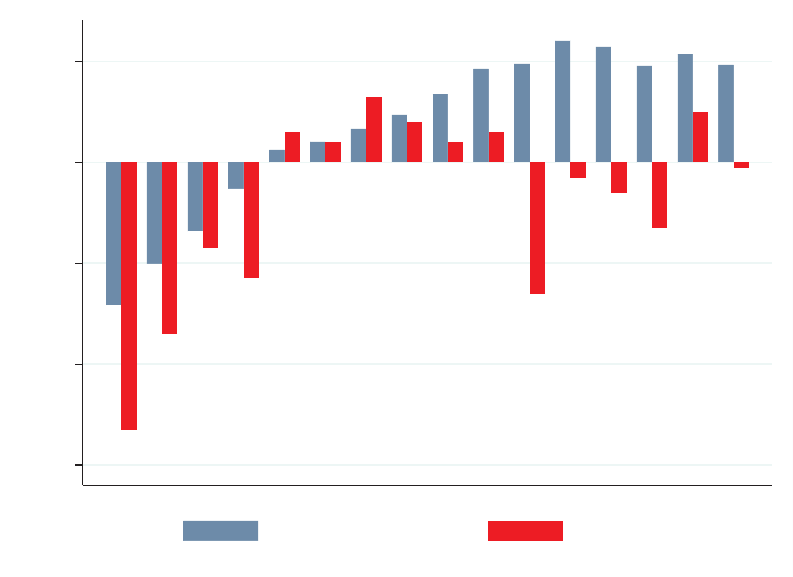
Figure 1: Greek GDP growth and CIPS GDP growth

Greek GDP growth (consta nt prices, seasonally adjusted) vs. weighted-average GDP growth

of CIPS (Cyprus, Italy, Portugal, Spain). Source: IMF.

-6

-4

-2

Percent

2013q1 2013q2 2013q3 2013q4 2014q1 2014q2 2014q3 2014q4 2015q1 2015q2 2015q3 2015q4 2016q1 2016q2 2016q3 2016q4

Weighted Avg. CIPS Greece

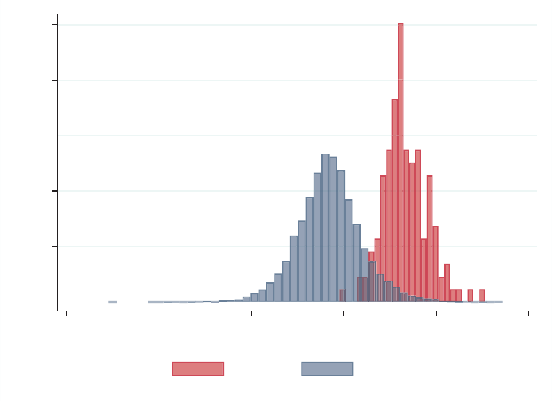
Figure 2: Sample distribution of log(Assets) vs. all Gr eek ﬁrms

This ﬁgure reports the distribution of log(Assets) for the 150 samp l e ﬁrms (red) and all

23,835 Greek ﬁrms in the 2014 Amadeus d at a (blue).

Density

0 5 10 15 20 25

log(Assets)

Sample Amadeus

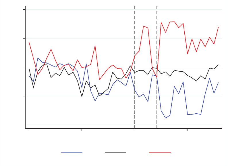
Figure 3: Time series of actual rates by initial breakeven rate

Corporate borrowers are divided into terciles according to each borrower’s i n i t i ally repo rt ed

breakeven rate in 2015. Each series plots the average a ct u al rate of the corresponding gr o u p

in the month. The ﬁrst vertical, dashed gray li n e denotes the beginning of 2015 , and the

second vertical, dash ed gray line denotes the introduction of capital controls in June 2015.

Average Interest Rate (%)

2013m1 2014m1 2015m1 2016m1

Date

Low Med High

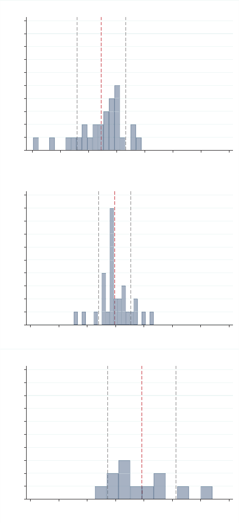
Figure 4: Actual rate changes by initial breakeven rate

These ﬁgures repo r t the distribution of actual rate changes by initial breakeven r a te. The

sample is divided into three terciles, according to the initially reported breakeven rate of

each corporate borrower in 2015 . Each plot shows a histogram of the changes to a borrower’s

actual rat es from 2014 to 2015 for the correspondi n g tercile of initial breakeven rate. The

red, vertical dashed lines represent the mean of each distribution , and the vertical, gray

dashed lines denot e the one-standard-deviation range around the mean.

Frequency

-6 -4 -2 0 2 4 6 8

Change in actual rate

Low

Frequency

-6 -4 -2 0 2 4 6 8

Change in actual rate

Med

Frequency

-6 -4 -2 0 2 4 6 8

Change in actual rate

High

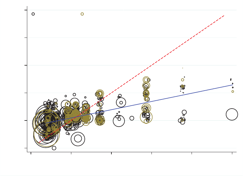
Figure 5: Actual rate and breakeven rate

This ﬁgure presents the scatter plot of actual and breakeven interest rates for n ew loans

from 2015 to June 2017. The red dashed line corr esponds to the 45

◦

line. The blue solid

line notes the OLS ﬁtted line. Th e size of the circle corresponds to the relati ve size of the

account. Black circles correspond to term loans an d brown circles correspond to credit lines.

Actual Rate

0 5 10 15 20 25

Breakeven Rate

Term Loans Credit Lines

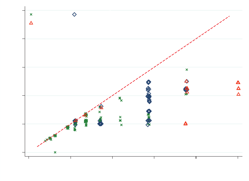
Figure 6: Reasons provided for below-breakeven-rate loans

Actual and breakeven rat es of below-breakeven-rate loans, grouped by the cited discount

reason. The red dashed line correspo n d s to the 45

◦

line.

0 5 10 15 20 25

Actual Rate

0 5 10 15 20 25

Breakeven Rate

Reason 1 Reason 2

Reason 3

Table 1: Summary sta ti s tics

This table reports the summary statistics. Panel A reports the loan-level variables for th e

1625 loans opened from 2015 and until the end of our sample per i od (2017m6) described in

section 3.4, and Panel B reports the summary statistics for borrower-lev

el variab l es for the

150 bo r r owers in our main sampl e. Detailed variable deﬁnitions are provided in Table A1 in

the appendix.

Panel A: Loan-level variables

Count Mean St. Dev P5 P25 P 50 P75 P95

Actual Rate (%) 1625 5.38 1.71 2.47 4.65 5.48 6.10 7.85

Breakeven Rate (%) 1625 4.76 3.34 1.97 2.36 4.64 5.57 10.98

Dif (%) 1625 0.62 2.73 -3.57 -0.02 0.49 2.28 4.46

Loan Amount (million e) 1625 3.62 14.35 0.04 0.20 0. 90 2.50 10.04

Maturity (years) 1581 0.62 1.51 0.08 0.17 0.25 0.50 1.99

Collateralized (%) 1625 85.17 35.55 0.00 100.00 100.00 100.00 100.00

Panel B: Borrower-level variables

Mean St. Dev P5 P25 P50 P75 P95

OROA (%) 4.59 5.97 -5.14 1.16 4.65 7.41 15.40

Deposits (million e) 18.88 81.72 0.38 1.48 4. 18 9.18 58.11

Total Asset s (million e) 237.88 655.06 15.86 43.02 78.35 175.72 832.10

Liabilities/Assets (%) 50.87 22.59 13.59 34.13 49.82 64.64 92.07

Table 2: Introduct io n of the new pricing guidelines and actual rate changes

This table reports the estimates of equation (18) in Panel A and equation (19) in Panel B.

The dependent variable in Panel A is the change i n the bo r r ower’s average interest rate from

2014 to 2015. The dependent variable in Panel B is the diﬀerence between the borrower’s

average 2015 breakeven rate and their average 2014 interest rate. Deposits and Assets are

in natural logarithms. In Panel A, OROA, Deposit s, Assets, and Liabilities/Assets are in

ﬁrst diﬀerences. Robust standard error s a re reported in pa r entheses. *, **, and *** in d i cat e

signiﬁcance at the 10%, 5%, and 1% l evel, respectively.

Panel A: First diﬀerence

2015

- AR

2014

(1) (2) (3)

Breakeve n

2015

- AR

2014

0.403

∗∗∗

0.397

∗∗∗

0.409

∗∗∗

(0.053) (0.055) (0.060)

∆ OROA

2015

-0.055 -0.048

(0.035) (0.040)

∆ Deposits

2015

0.287

∗

0.263

(0.166) (0.173)

∆ Assets

2015

-0.344 -0.676

(0.990) (1.094)

∆ Liabilities/Assets

2015

-0.006 -0.003

(0.008) (0.009)

Observations 70 65 63

0.627 0.665 0.696

Industry FE No No Yes

Panel B: Levels

Actual Rate

2015

(1) (2) (3)

Breakeven

2015

0.379

∗∗∗

0.372

∗∗∗

0.377

∗∗∗

(0.033) (0.039) (0.042)

Actual Rate

2014

0.051 0.089 0.108

(0.152) (0.158) (0.171)

OROA -0.007 -0.005

(0.023) (0.022)

Deposits 0.023 -0.000

(0.086) (0.088)

Assets 0.127 0.137

(0.154) (0.174)

Liabilities/Assets 0.008 0.007

(0.006) (0.007)

Observations 70 67 65

0.725 0.744 0.763

Industry FE No No Yes

Table 3: Lasso reg res s ions with board-characteristic variables

This table reports the OLS r egressi on and post-lasso regression using board-characteristic variables, sepa-

rately for the pre-guideline period (Pre-BE) and post-guideline period (Post-BE). The dependent variable

is the actual interest rate of each loan (in all columns). All variables are standardized to have zero mean

and a standard deviation of one. For each sample peri od, the ﬁ rs t column reports the OLS r esul t s with the

full set of board-characteristic variables. To obtain the post-lasso results in the latter column, we ﬁrst run

a lasso regression with all covariates after partialling out quarter ﬁxed eﬀects. The tuning parameter λ is

chosen , where the mean-squared prediction error (MSPE ) i s hi ghest but still within one standard error of the

minimum MSPE (i.e., the “one standard error rule”) using 10-fold cross-validation. Finally, we run an OLS

regression using the covariates selected by the lasso. Deposits and Assets are in logs. Board -characteristic

variables are deﬁned in the Appendix, Table A1. Standard errors are clustered by borrower, and reported

n parentheses. *, **, and *** indicate signiﬁcance at the 10%, 5%, and 1% level, respectively.

Pre-BE Post-BE

(1) (2) (3) (4)

OLS post-lasso OLS post-lasso

Breakeven Rate 0.025 -0.004 0.617

∗∗∗

0.663

∗∗∗

(0.090) (0.107) (0.087) (0.066)

OROA 0.016 -0.050

(0.094) (0.058)

Deposits -0.015 -0.087

(0.134) (0.088)

Assets -0.059 -0.120 0.073

(0.165) (0.123) (0.117)

Liabilities/Assets 0.017 0.009 0.002

(0.082) (0.083) (0.069)

Maturity -0.031 -0.000

(0.030) (0.024)

Collateral 0.054 0.090 0.021

(0.068) (0.060) (0.042)

founder on board -0.290

∗∗

-0.168

∗∗∗

-0.011

(

0.114) (0.063) (0.070)

founder is CEO 0.146 0.037

(0.103) (0.087)

founder’s family on board -0.013 0.130

∗

(0.101) (0.070)

amily equity ownership 0.124 0.065 -0.118

(0.102) (0.063) (0.079)

bank executive on board 0.475

∗∗∗

0.476

∗∗∗

0.039

(

0.149) (0.139) (0.059)

media executive on board 0.237

∗∗∗

0.212

∗∗∗

0.095

∗∗∗

(0.041) (0.025) (0.022)

olitician on board -0.398

∗∗∗

-0.397

∗∗∗

-0.043

(0.124) (0.127) (0.075)

politician family on board 0.209

∗∗

0.199

∗∗

0.045

(0.082) (0.079) (0.042)

bank executive senior manager -0.392

∗∗

-0.367

∗∗∗

-0.016

(

0.173) (0.132) (0.063)

Observations 1012 1012 1194 1194

0.312 0.306 0.488 0.463

uarter FE Yes Yes Yes Yes

Table 4: Actual rate and breakeven rate

This table reports the ba sel i n e estimates of equation (20), where columns (1)-(5) incremen-

tally add covariates. Column (6) report s the results from augmenting equation (20 ) with

ﬁrm-ﬁxed eﬀects. The dependent variable is the actual interest rate of each loan (in all

columns). Deposits and Assets are in natur al logarithms. Standard errors, whi ch are clus-

tered by borrower, are reported in parent h eses. *, **, and *** i n d i ca t e signiﬁcance at the

10%, 5%, and 1% level, respectively.

(1) (2) (3) (4) (5) (6)

Breakeven Rate 0.299

∗∗∗

0.310

∗∗∗

0.285

∗∗∗

0.293

∗∗∗

0.282

∗∗∗

0.095

(0.033) (0.031) (0.035) (0.039) (0.038) (0.097)

OROA -0.016 -0.017 -0.026

∗

(0.019) (0.019) (0.016)

Deposits -0.076 -0.050 -0.151

∗∗

(0.088) (0.090) (0.062)

Assets 0.082 0.048 0.224

∗∗

(0.132) (0.132) (0.096)

Liabilities/Assets 0.004 0.003 0.001

(0.006) (0.006) (0.006)

Maturity -0.072 -0.007 -0.004

(0.065) (0.044) (0.042)

Collateral 0.262 0.034 -0.249

(0.193) (0.163) (0.271)

Observations 1625 1625 1571 1529 1486 1549

0.339 0.389 0.390 0.395 0. 442 0.601

Quarter FE No Yes Yes Yes Yes Yes

Industry FE No No No No Yes No

Firm FE No No No No No Yes

Table 5: Lagged interest rates

This table augments equation (20) with a lagged actual rate. Speciﬁcally, Actual Rate

t−1

calculated as th e average interest rate of the borr ower’s loan s in the most recent previous

month. Columns (1)-(5) incrementally add the covar i a tes of the speciﬁcation, and column

(6) includ es ﬁrm ﬁxed eﬀect s. Deposits and Assets are in n at u r a l logarithms. Standard

errors, which a re clustered by borrower, are reported in parentheses. *, **, and *** indicate

signiﬁcance of 10%, 5%, and 1% level, respectively.

(1) (2) (3) (4) (5) (6)

Breakeven Rate 0.186

∗∗∗

0.199

∗∗∗

0.184

∗∗∗

0.193

∗∗∗

0.198

∗∗∗

0.079

(0.042) (0.042) (0.042) (0.045) (0.039) (0.108)

Actual Rate

t−1

0.567

∗∗∗

0.556

∗∗∗

0.580

∗∗∗

0.583

∗∗∗

0.537

∗∗∗

0.523

∗∗∗

(0.093) (0.091) (0.072) (0.074) (0.060) (0.105)

OROA -0.012 -0.011 -0.014

(0.015) (0.016) (0.013)

Deposits 0.053 0.070 -0.021

(0.078) (0.077) (0.066)

Assets 0.063 0.049 0.232

∗∗

(0.098) (0.096) (0.094)

Liabilities/Assets 0.002 0.002 0.001

(0.005) (0.005) (0.005)

Maturity -0.011 -0.013 -0.009

(0.059) (0.057) (0.075)

Collateral 0.169 -0.013 -0.247

(0.158) (0.162) (0.287)

Observations 1423 1423 1389 1364 1331 1376

0.447 0.488 0.490 0.498 0. 527 0.614

Quarter FE No Yes Yes Yes Yes Yes

Industry FE No No No No Yes No

Firm FE No No No No No Yes

Table 6: Asymmetric pa s s -thro ugh

The dependent variable is the actual rate of each loan in all columns. Columns (1)-(2)

only includ e borrowers whose ﬁrst reported brea keven rate in 2015 is below the median

breakeven rate of initial breakeven rates. Columns (3)-(4) only include the borrowers who se

ﬁrst reported 2015 breakeven rate is above the median of initial breakeven rates. S t a n d ar d

errors, which a re clustered by borrower, are reported in parentheses. *, **, and *** indicate

signiﬁcance at the 10%, 5%, and 1% l evel, respectively.

Below-med ian BE Above-median BE

(1) (2) (3) (4)

Breakeven Rate 0.434

∗∗

0.432

∗∗

0.041 0.044

(0.190) (0.180) (0.093) (0.092)

Maturity 0.082

∗∗

-0.083

(0.039) (0.079)

Collateral -0.260 0.043

(0.232) (0.231)

Observations 544 532 883 863

0.480 0.496 0.411 0.432

Quarter FE Yes Yes Yes Yes

Industry FE No No No No

Firm FE Yes Yes Yes Yes

Table 7: Future borrower credit rating

This tab l e reports the results from estimating equation (21). The dependent variable in all

columns is a borrower’s rating 12 month s lat er . Diﬀ

for a borrower i in month t is calculated

as the average acr oss all of the borrower’s loans’ actual - breakeven rate in t. Column (1)

shows the result for a l l observations. Co l u m n (2) only includes observations with negative

Diﬀ

, and colu m n (3) only includes ob ser vations with positive Diﬀ

. A lower value of the

ariable ”Rating” corresponds to better credit quality. Standard errors are clustered by

borrower, and reported in parentheses. *, **, and *** i n d i ca t e signiﬁcance at the 10%, 5%,

and 1% level, respectively.

(1) (2) (3)

All Customers Negative Dif Positive Dif

Dif -0.084 -0.070 0.006

(0.068) (0.134) (0.135)

Rating 0.704

∗∗∗

0.705

∗∗∗

0.690

∗∗∗

(0.092) (0.201) (0.094)

Observations 465 123 342

0.519 0.631 0.396

Quarter FE Yes Yes Yes

Industry FE Yes Yes Yes

Firm FE No No No

Table 8: Regulatory cos ts and actual rate

This table reports the resu l t s from augmenting the baseline equation (20) with regulatory

capital costs. Columns (1)-(2) include al l accounts, and column (3) incl u d es term loans

only. Column (4) only includes new credit term loans, which are deﬁned as an a ccou nt that

increases the borrower’s t o ta l outsta n d i n g balan ce by at least 10%. The dependent variable

is a loan’s interest rate in all columns. Deposits and Assets are in natu ra l logarithms.

Standard errors are clustered by borrower, and reported in parentheses. *, **, an d ***

indicate signiﬁcance at t h e 10%, 5%, and 1% l evel, respectively.

(1) (2) (3) (4)

Term Loans New Credit Term Loans

Breakeve n Rate 0.248

∗∗∗

0.277

∗∗∗

0.244

∗∗

0.268

∗∗∗

(0.083) (0.080) (0.098) (0.092)

Regulatory Capital Cost 0.124 0.042 0.112 -0.007

(0.732) (0.643) (0.910) (0.887)

OROA -0.027 -0.026 -0.033

∗

-0.018

(0.018) (0.016) (0.017) (0.027)

Deposits -0.157

∗∗

-0.151

∗∗

-0.181

∗∗

-0.100

(0.064) (0.061) (0.079) (0.144)

Assets 0.229

∗∗

0.225

∗∗

0.268

∗∗

0.217

(0.104) (0.098) (0.126) (0.172)

Liabilities/Assets 0.003 0.001 0.001 0.005

(0.006) (0.006) (0.007) (0.008)

Maturity 0.023 -0.007 0.043 0.047

(0.040) (0.044) (0.040) (0.065)

Collateral 0.075 0.037 -0.070 -0.108

(0.174) (0.158) (0.223) (0.335)

Observations 1486 1486 1054 296

0.397 0.442 0.389 0.438

Quarter FE No Yes No No

Industry FE Yes Yes Yes Yes

Firm FE No No No No

A Appendix

A.1 Proofs

Proof of Proposition 2. S

etting V

H,c

inside (9) and solving for R

H,c

leads to (13). To

prove R

L,c

= π

, we arg u e by contradiction. Indeed, suppose (counterfactually) R

L,c

< π

In that case, it must be that both in the L and the H regime the constraints V

H,c

≤

and V

L,c

≤

are both binding (because the bank is only constrained by the no-poaching

condition in ei th er regime). Accordingly, (10) implies

L,c

= (r + ρ)

− ρC

∗

. (23)

However, (7) implies

< r

∗

− p

(1 − C

∗

) . (

24)

But condition ( 11) together with (23) and (24) imply

< r

∗

− p

(1 − C

∗

) <

+ ρ



− C

∗



= R

L,c

This contradicts the assumption that R

L,c

< π

. T

herefore, it must be that R

L,c

= π

Using R

L,c

= π

inside (10) and using V

H,c

leads to (14). Assumption (12) implies

liquidation of the ﬁr m in the low regime i s not optimal.

Proof of Proposition 3. Proposition 2 implies

L,c

− R

H,c

ρ (1 − C

∗

)

− R

H,c

ρ (1 − C

∗

)

−

r +

(r + ρ)

− 1



+ p

− V

L,c



ρ (1 − C

∗

)

. (25)

Conditions (11) and (2 4) imply

< r

+ ρ



− C

∗



. (26)

Combini n g (25) with (26) leads to

L,c

− R

H,c

ρ (1 − C

∗

)

+ ρ

− C

∗



−

r + (r + ρ)

− 1



+ p

− V

L,c



ρ (1 − C

∗

)

ρ (1 − C

∗

) − p

− V

L,c



ρ (1 − C

∗

)

= 1 − p

− V

L,c



ρ (1 − C

∗

)

≤ 1,

where the last line follows from the no-poaching conditio n V

L,c

≤

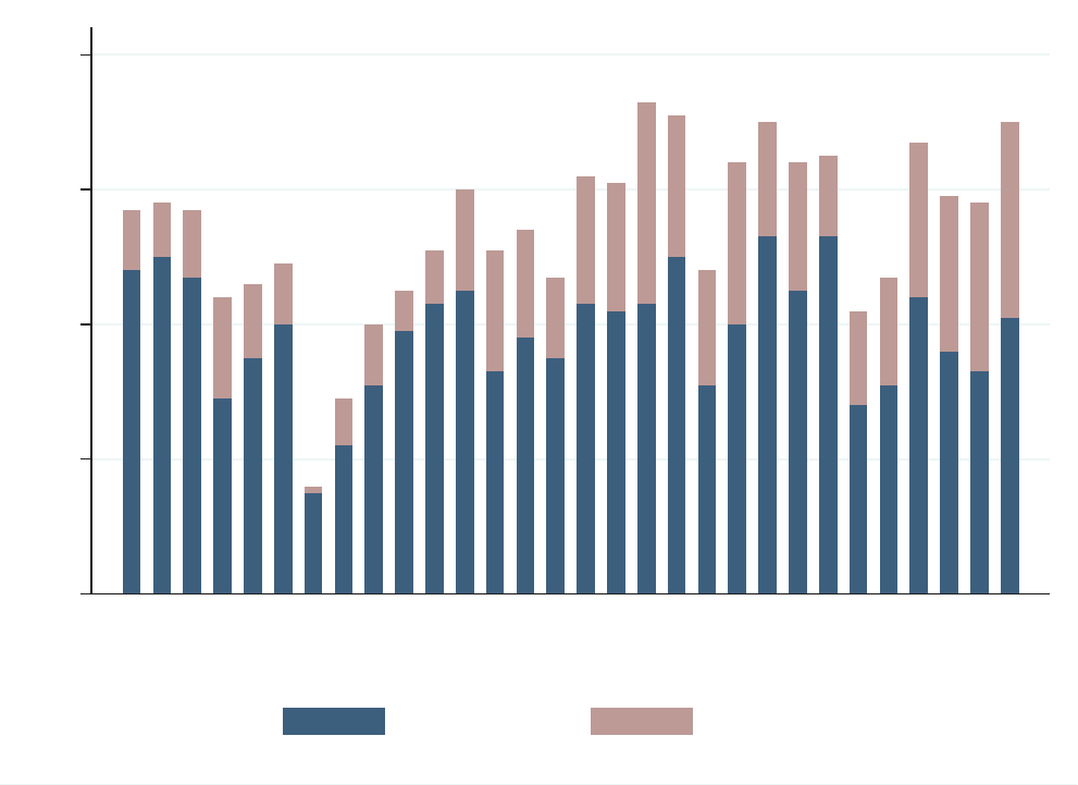
A.2 Additional ﬁgures and tabl es

Figure A1: New accounts by type

This ﬁgur e reports the number of new accounts by type – namel y, term l o an or credit lin e –

for each month in the sam p l e period. The dark-blue bars correspond to the number of new

term loans in the month, and the light-brown b a rs represent the number of new credit-line

accounts.

2015m1

2015m2

2015m3

2015m4

2015m5

2015m6

2015m7

2015m8

2015m9

2015m10

2015m11

2015m12

2016m1

2016m2

2016m3

2016m4

2016m5

2016m6

2016m7

2016m8

2016m9

2016m10

2016m11

2016m12

2017m1

2017m2

2017m3

2017m4

2017m5

2017m6

Term Loans Credit Lines

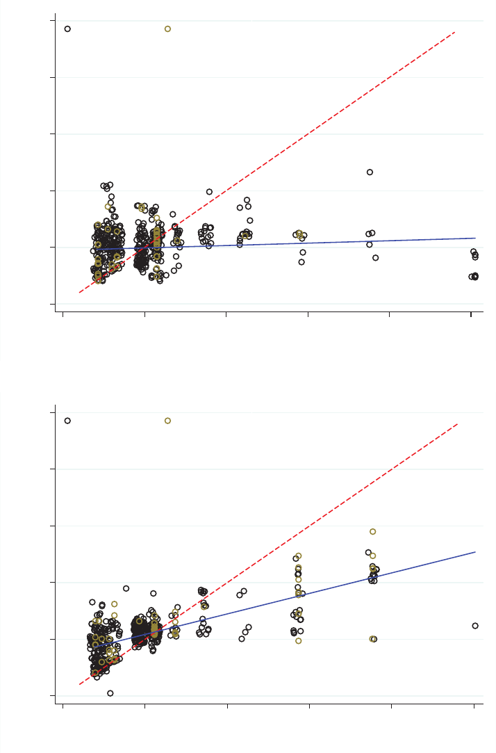
Figure A2: Actual rates and breakeven rates in 2014 and 2015

This ﬁgure shows the scatter plot of actual and breakeven rates for 2014 and 2015. The red dashed line

corresponds to the 45

◦

line. The blue solid line notes the OLS ﬁtted line. Black circles correspond to term

loans and brown circles correspond to credit lines.

Panel A: 2014

Actual Rate

0 5 10 15 20 25

Breakeven Rate

Term Loans Credit Lines

Panel B: 2015

Actual Rate

0 5 10 15 20 25

Breakeven Rate

Term Loans Credit Lines

Figure A3: Borrower composition

This ﬁgure shows borrower composition over the sample period. Th e ﬁgure includes 89

borrowers who receive a l o an in 2015 and furthermore appear in the sam p l e in at least two

separate quarters. For each borrower, ﬁ l l ed boxes represent the quarters in whi ch they open

a new loan with the bank. Each borrower is color coded such that dark r ed correspond s

to borrowers who receive an upward breakeven-rate ad ju st ment, li ght pink corresponds to

borrowers who receive a downward breakeven-rate adjustment, and medium red corresponds

to those who do not receive any adjustment.

2015q1 2015q2 2015q3 2015q4 2016q1 2016q2 2016q3 2016q4 2017q1 2017q2

Date

customerid

No loan BE change < 0 BE change = 0 BE change > 0

Figure A4: [Continued] Borrower composition

This ﬁgure shows borrower composition over the sample period. Th e ﬁgure includes 89

borrowers who receive a lo an in 2015 and fu r t her m or e appear in the sample i n at least

two separate quarters. For each b o r r ower, ﬁlled boxes represent the quarters in which they

open a new loan with the bank. The sample borrowers are divided into th r ee tercile groups

according to their ini t i al Diﬀ, namely, the diﬀer en ce between the actual interest rate and

breakeven rate. Each borrower is color coded such that dark red corresponds to borrowers

in the top tercile, mediu m red correspon d s to the middle tercile, and light pink corresponds

to the bott o m tercile.

2015q1 2015q2 2015q3 2015q4 2016q1 2016q2 2016q3 2016q4 2017q1 2017q2

Date

customerid

No loan Low Dif Med Dif High Dif

Table A1: Variable deﬁnitions

Variable Deﬁnition

Borrower-level Variables

OROA Deﬁned as EBIT/(Total Assets)

Deposits Reported in euros

Assets Reported in euros

Liabilities/Assets Deﬁned as (Current Liabilities)/(Total Assets)

Industry

Rating The bank’s credit rating of the borrower; lower rating corresponds to

higher credit quality.

Loan-level Variab l es

Actual Rate Interest rate of t h e loan.

Breakeven Rate The breakeven interest rate for the loan as computed by the bank’s

own pricing department.

Diﬀ Deﬁned as actual rate − breakeven rate.

Loan Amount Reported in euros.

Maturity Maturity of the l oan in years at issuance.

Collateralization An indicator variable that takes a value 1 if the loan belongs to a

borrower who has provided collateral in that month

Board-Characteristic Variables

founder on board The founder is on the board

founder is CEO The founder is the CEO

founder’s family on board Th e founder’s family memb er is on the board

family equity ownership The founder family’s ownership of outstanding equity

bank executive on boar d Number of board members who are or were bank executives

media executive on board Number of board member s who are or wer e media executives

politician on board Number of board members who have or had political aﬃliations

politician family on board Number of board member s who have family members with pol i t i cal

aﬃliations

bank executive senior man ager Has a senior manager who was a bank executive

Table A2: Summary sta ti s ti cs by breakeven rate - actual rate diﬀerence

This table reports the summar y statistics for loan-level variables and borrower-level variables

in our main samp l e. Detailed variable deﬁnitions are provided in Table A1. Panel A reports

he summary statist i cs only for loans with a rate higher t h a n their breakeven rate. Panel

B reports the results only for below-breakeven loans. S i m i l ar l y, Panel C only includes the

borrowers who never receive a below-breakeven loan from 2015 and until the en d of our

sample period (2017m6), and Panel D only includes the borrowers who receive at least one

below-breakeven loan.

Panel A: Above-breakeven loans

Count Mean St. Dev P5 P25 P50 P75 P95

Actual Rate (%) 1211 5.22 1.52 2.36 4.59 5.55 6.10 7.60

Breakeven Rate (%) 1211 3.56 1.52 1.97 2.21 2.81 4.64 5. 57

Dif (%) 1211 1.66 1.52 0.10 0.35 1.21 2.63 4.63

Loan Amount (million e) 1211 3.86 16.07 0.04 0.20 0.86 2.33 10.09

Maturity (years) 1181 0.58 1.49 0.08 0.13 0.25 0.50 2.01

Collateralized (%) 1211 83.90 36.77 0.00 100.00 100.00 100.00 100.00

Panel B: Below-breakeven loans

Count Mean St. Dev P5 P25 P 50 P75 P95

Actual Rate (%) 414 5.87 2.11 2.90 5.01 5.41 6.17 11.02

Breakeven Rate (%) 414 8.27 4.54 3.13 5.57 6.83 8.57 18.85

Dif (%) 414 -2.40 3.20 -8.73 -3.57 -1.34 -0.23 -0.06

Loan Amount (million e) 414 2.93 7.19 0.03 0.20 1.00 2.87 10.01

Maturity (years) 400 0.76 1.54 0.08 0.23 0.41 0.75 1.88

Collateralized (%) 414 88.89 31.46 0.00 100.00 100.00 100.00 100.00

Panel C: Above-breakeven borrowers

Mean St. Dev P5 P25 P50 P75 P95

OROA (%) 6.85 5.87 -0.17 3.01 5.79 9.58 17.04

Deposits (million e) 24.94 118.53 0.51 1.36 3.82 7.10 28.22

Total Asset s (million e) 263.56 939.87 13.47 33.88 65.75 106.65 531.45

Liabilities/Assets (%) 50.33 21.17 14.74 32.35 50.83 62.27 84.80

Panel D: Below-breakeven borrowers

Mean St. Dev P5 P25 P50 P75 P95

OROA (%) 2.88 5.48 -6.72 -0.79 3.12 6.17 11.85

Deposits (million e) 14.31 34.11 0.21 1.48 4.43 10.20 69.04

Total Asset s (million e) 218.37 300.20 21.95 55.62 116.65 278.67 865.85

Liabilities/Assets (%) 51.27 23.74 9.85 35.27 49.74 65.94 92.63

Table A3: Summary st a ti s tics for account-level variables, term loans

This table reports the summary statisti cs for the account-level variables in Table 1, but only

for term loans.

Panel A: All accounts

Count Mean St. Dev P5 P25 P 50 P75 P95

Actual Rate (%) 1163 5.21 1.76 2.36 4.45 5.25 6.10 7.85

Breakeven Rate (%) 1163 4.36 3.41 1.97 2.21 3.13 5.57 10.98

Dif (%) 1163 0.85 2.82 -3.57 0.12 0.72 2.53 4.63

Loan Amount (million e) 1163 4.59 16.68 0.05 0.30 1.00 3.01 16.83

Maturity (years) 1143 0.71 1.76 0.08 0.09 0.25 0.50 3.01

Collateralized (%) 1163 83.40 37.22 0.00 100.00 100.00 100.00 100.00

Panel B: Above-breakeven accounts

Count Mean St. Dev P5 P25 P50 P75 P95

Actual Rate (%) 932 5.05 1.53 2.35 4.10 5.20 6.06 7.60

Breakeven Rate (%) 932 3.30 1.39 1.97 2.21 2.57 4.64 5.57

Dif (%) 932 1.75 1.53 0.08 0.43 1.32 2.79 4.63

Loan Amount (million e) 932 4.63 18.05 0.05 0.30 1.00 2.90 16.49

Maturity (years) 917 0.66 1.68 0.08 0.09 0.25 0.50 3.00

Collateralized (%) 932 82.73 37.82 0.00 100.00 100.00 100.00 100.00

Panel C: Below-breakeven accounts

Count Mean St. Dev P5 P25 P50 P75 P95

Actual Rate (%) 231 5.87 2.37 2.38 4.84 5.47 6.58 11.02

Breakeven Rate (%) 231 8.67 5.26 2.57 5.57 6.83 10.98 18. 85

Dif (%) 231 -2.81 3.73 -12.35 -4.07 -1.07 -0.23 -0.03

Loan Amount (million e) 231 4.44 9.28 0.04 0.50 2.00 3.65 24.18

Maturity (years) 226 0.90 2.02 0.08 0.22 0.26 0.50 4.58

Collateralized (%) 231 86.15 34.62 0.00 100.00 100.00 100.00 100.00

Table A4: Summary st a ti s tics for account-level variables, credit lines

This table reports the summary statisti cs for the account-level variables in Table 1, but only

for credit-line accou nts.

Panel A: All accounts

Count Mean St. Dev P5 P25 P 50 P75 P95

Actual Rate (%) 462 5.82 1.51 3.26 5.25 5.59 6.42 8.90

Breakeven Rate (%) 462 5.76 2.94 2.21 4.64 5.57 6.83 8.57

Dif (%) 462 0.06 2.40 -3.57 -1.30 0.14 1.14 4.46

Loan Amount (million e) 462 1.18 3.94 0.03 0.11 0.31 1.16 3.95

Maturity (years) 438 0.41 0.27 0.14 0.21 0.38 0.41 0.96

Collateralized (%) 462 89.61 30.55 0.00 100.00 100.00 100.00 100.00

Panel B: Above-breakeven accounts

Count Mean St. Dev P5 P25 P50 P75 P95

Actual Rate (%) 279 5.79 1.35 3.15 5.52 5.71 6.76 7.85

Breakeven Rate (%) 279 4.45 1.61 1.97 2.81 5.57 5.57 5.57

Dif (%) 279 1.34 1.44 0.12 0.14 0.94 2.28 4.46

Loan Amount (million e) 279 1.29 4.95 0.03 0.11 0.26 0.86 3.95

Maturity (years) 264 0.30 0.16 0.13 0.21 0.23 0.38 0.50

Collateralized (%) 279 87.81 32.77 0.00 100.00 100.00 100.00 100.00

Panel C: Below-breakeven accounts

Count Mean St. Dev P5 P25 P 50 P75 P95

Actual Rate (%) 183 5.87 1.72 5.00 5.25 5.40 5.51 10.25

Breakeve n Rate (%) 183 7.75 3.36 5.57 5.57 6.83 8.57 14.33

Dif (%) 183 -1.88 2.26 -6.49 -2.06 -1.43 -0.20 -0.06

Loan Amount (million e) 183 1.02 1.40 0.02 0.11 0.45 1.37 3.99

Maturity (years) 174 0.57 0.31 0.19 0.38 0.41 0.94 0.96

Collateralized (%) 183 92.35 26.65 0.00 100.00 100.00 100.00 100.00

Table A5: Actual rat e and breakeven rate, term loans

The following table presents the results from regressions of actual rate on breakeven rate as

in Table 4, but for term loans on l y.

(1) (2) (3) (4) (5) (6)

Breakeven Rate 0.292

∗∗∗

0.309

∗∗∗

0.289

∗∗∗

0.294

∗∗∗

0.283

∗∗∗

0.066

(0.037) (0.034) (0.043) (0. 045) (0.044) (0.067)

OROA -0.023 -0.023 -0.030

∗∗

(0.018) (0.018) (0.015)

Deposits -0.014 -0.002 -0.162

∗∗

(0.096) (0.103) (0.078)

Assets 0.038 0.017 0.234

∗

(0.139) (0.139) (0.119)

Liabilities/Assets 0.004 0.003 -0.001

(0.007) (0.006) (0.006)

Maturity -0.061 0.001 -0.018

(0.071) (0.046) (0.049)

Collateral 0.173 -0.121 -0.421

(0.226) (0.193) (0.355)

Observations 1163 1163 1114 1095 1054 1112

0.320 0.400 0.402 0.404 0. 455 0.631

Quarter FE No Yes Yes Yes Yes Yes

Industry FE No No No No Yes No

Firm FE No No No No No Yes

Table A6: Actual rat e and breakeven rate, credit lines

The following table presents the results from regressions of actual rate on breakeven rate as

in Table 4, but for credit line a ccounts only.

(1) (2) (3) (4) (5) (6)

Breakeve n Rate 0.298

∗∗∗

0.304

∗∗∗

0.230

∗∗∗

0.237

∗∗

0.208

∗

0.187

(0.064) (0.067) (0.049) (0.088) (0.110) (0.194)

OROA 0.047 0.068 0.066

(0.047) (0.087) (0.097)

Deposits -0.492

∗∗∗

-0.499

∗

-0.513

(0.149) (0.276) (0.330)

Assets 0.439

∗∗∗

0.467 0.414

(0.156) (0.277) (0.307)

Liabilities/Assets 0.009 0.020 0.026

(0.010) (0.016) (0.020)

Maturity -0.094 -0.044 2.495

(1.001) (1.059) (1.973)

Collateral 1.001

∗∗

0.627

∗∗

0.129

(0.341) (0.282) (0.303)

Observations 462 462 457 434 432 437

0.338 0.381 0. 440 0.482 0.489 0.569

Quarter FE No Yes Yes Yes Yes Yes

Industry FE No No No No Yes No

Firm FE No No No No No Yes